as z%E2%86%920
(0.002 seconds)
31—40 of 734 matching pages
31: 10.13 Other Differential Equations
…
►
10.13.5
,
…
►
10.13.7
,
…
►In (10.13.9)–(10.13.11) , are any cylinder functions of orders , respectively, and .
►
10.13.9
,
►
10.13.10
,
…
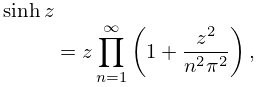
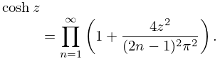
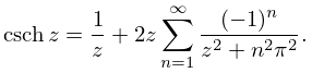
32: 4.36 Infinite Products and Partial Fractions
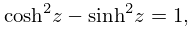
33: 4.35 Identities
34: 10.49 Explicit Formulas
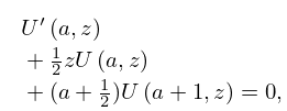
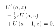
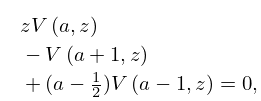
35: 12.8 Recurrence Relations and Derivatives
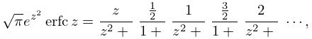
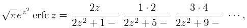
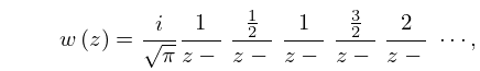
36: 7.9 Continued Fractions
37: 10.72 Mathematical Applications
…
►The number can also be replaced by any real constant
in the sense that
is analytic and nonvanishing at ; moreover, is permitted to have a single or double pole at .
…
►In regions in which the function has a simple pole at and is analytic at (the case in §10.72(i)), asymptotic expansions of the solutions of (10.72.1) for large can be constructed in terms of Bessel functions and modified Bessel functions of order , where is the limiting value of as .
…
►In (10.72.1) assume and depend continuously on a real parameter , has a simple zero and a double pole , except for a critical value , where .
Assume that whether or not , is analytic at .
…These approximations are uniform with respect to both and , including , the cut neighborhood of , and .
…
38: 7.1 Special Notation
…
►
►
…
►The main functions treated in this chapter are the error function ; the complementary error functions and ; Dawson’s integral ; the Fresnel integrals , , and ; the Goodwin–Staton integral ; the repeated integrals of the complementary error function ; the Voigt functions and .
►Alternative notations are , , , , , , , .
►The notations , , and are used in mathematical statistics, where these functions are called the normal or Gaussian probability functions.
…
| real variable. | |
| complex variable. | |
| … | |
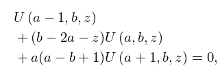
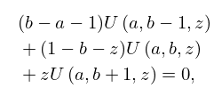
39: 13.3 Recurrence Relations and Derivatives
40: 15.5 Derivatives and Contiguous Functions
…
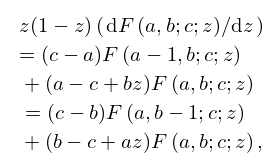
►
15.5.5
…
►
15.5.10
.
…
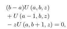
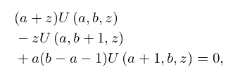
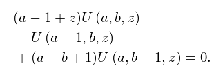
►The six functions , , are said to be contiguous to .
…
►By repeated applications of (15.5.11)–(15.5.18) any function , in which are integers, can be expressed as a linear combination of and any one of its contiguous functions, with coefficients that are rational functions of , and .
…
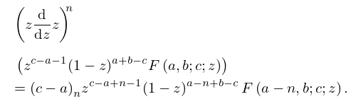
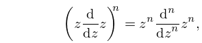
►
15.5.20
…
