as x→±1

SearchAdvancedHelp

(0.042 seconds)

21—30 of 629 matching pages

21: 10.63 Recurrence Relations and Derivatives

… ►

$f_{\nu +1}(x)+g_{\nu +1}(x)-f_{\nu -1}(x)-g_{\nu -1}(x)=2\sqrt{2}{f}_{\nu }^{\prime }(x),$

… ►

$f_{\nu }^{\prime }(x)=(1/\sqrt{2})\left(f_{\nu +1}(x)+g_{\nu +1}(x)\right)+(\nu /x)f_{\nu }(x).$

►

$\sqrt{2}{\mathrm{ber}}^{\prime }x={\mathrm{ber}}_{1}x+{\mathrm{bei}}_{1}x,$

►

$\sqrt{2}{\mathrm{bei}}^{\prime }x=-{\mathrm{ber}}_{1}x+{\mathrm{bei}}_{1}x.$

►

$\sqrt{2}{\ker }^{\prime }x={\ker }_{1}x+{\mathrm{kei}}_{1}x,$

…

22: 8.26 Tables

… ►

Zhang and Jin (1996, Table 3.8) tabulates $\gamma (a,x)$ for $a=0.5,1,3,5,10,25,50,100$, $x=0(.1)1(1)3,5(5)30,50,100$ to 8D or 8S.

… ►

Abramowitz and Stegun (1964, pp. 245–248) tabulates $E_n\left(x\right)$ for $n=2,3,4,10,20$, $x=0(.01)2$ to 7D; also $(x+n){\mathrm{e}}^x{E}_n\left(x\right)$ for $n=2,3,4,10,20$, $x^{-1}=0(.01)0.1(.05)0.5$ to 6S.

… ►

Pagurova (1961) tabulates $E_n\left(x\right)$ for $n=0(1)20$, $x=0(.01)2(.1)10$ to 4-9S; ${\mathrm{e}}^x{E}_n\left(x\right)$ for $n=2(1)10$, $x=10(.1)20$ to 7D; ${\mathrm{e}}^x{E}_p\left(x\right)$ for $p=0(.1)1$, $x=0.01(.01)7(.05)12(.1)20$ to 7S or 7D.

►

Stankiewicz (1968) tabulates $E_n\left(x\right)$ for $n=1(1)10$, $x=0.01(.01)5$ to 7D.

►

Zhang and Jin (1996, Table 19.1) tabulates $E_n\left(x\right)$ for $n=1,2,3,5,10,15,20$, $x=0(.1)1,1.5,2,3,5,10,20,30,50,100$ to 7D or 8S.

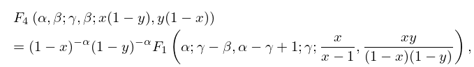
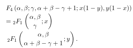
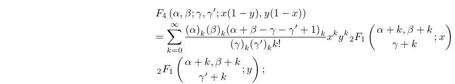
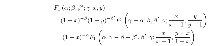
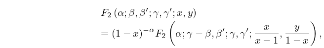
23: 16.16 Transformations of Variables

… ►

16.16.5_5 $$F_4(\alpha ,\beta ;\gamma ,\beta ;x(1-y),y(1-x))={(1-x)}^{-\alpha }{(1-y)}^{-\alpha }{F}_1(\alpha ;\gamma -\beta ,\alpha -\gamma +1;\gamma ;\frac{x}{x-1},\frac{xy}{(1-x)(1-y)}),$$

ⓘ

Symbols:

$F_1(\alpha ;\beta ,{\beta }^{\prime };\gamma ;x,y)$: first Appell function and $F_4(\alpha ,\beta ;\gamma ,{\gamma }^{\prime };x,y)$: fourth Appell function

Referenced by:

§16.16(i), Erratum (V1.1.12) for Additions

Permalink:

http://dlmf.nist.gov/16.16.E5_5

Encodings:

pMML, png, TeX

Addition (effective with 1.1.12):

This equation was added.

See also:

Annotations for §16.16(i), §16.16 and Ch.16

►

16.16.6 $$F_4(\alpha ,\beta ;\gamma ,\alpha +\beta -\gamma +1;x(1-y),y(1-x))={}_2{}^{}F_1^{}(\genfrac{}{}{0pt}{}{\alpha ,\beta }{\gamma };x){}_2{}^{}F_1^{}(\genfrac{}{}{0pt}{}{\alpha ,\beta }{\alpha +\beta -\gamma +1};y).$$

ⓘ

Symbols:

$F_4(\alpha ,\beta ;\gamma ,{\gamma }^{\prime };x,y)$: fourth Appell function and ${}_2{}^{}F_1^{}(a,b;c;z)$: $=F(a,b;c;z)$ notation for Gauss’ hypergeometric function

Referenced by:

§16.16(i)

Permalink:

http://dlmf.nist.gov/16.16.E6

Encodings:

pMML, png, TeX

See also:

Annotations for §16.16(i), §16.16 and Ch.16

… ►

16.16.7 $$F_4(\alpha ,\beta ;\gamma ,{\gamma }^{\prime };x(1-y),y(1-x))=\sum _{k=0}^{\mathrm{\infty }}\frac{{\left(\alpha \right)}_k{\left(\beta \right)}_k{\left(\alpha +\beta -\gamma -{\gamma }^{\prime }+1\right)}_k}{{\left(\gamma \right)}_k{\left({\gamma }^{\prime }\right)}_{k}k!}{x}^k{y}^k{}_2{}^{}F_1^{}(\genfrac{}{}{0pt}{}{\alpha +k,\beta +k}{\gamma +k};x){}_2{}^{}F_1^{}(\genfrac{}{}{0pt}{}{\alpha +k,\beta +k}{{\gamma }^{\prime }+k};y);$$

ⓘ

Symbols:

$F_4(\alpha ,\beta ;\gamma ,{\gamma }^{\prime };x,y)$: fourth Appell function, ${}_2{}^{}F_1^{}(a,b;c;z)$: $=F(a,b;c;z)$ notation for Gauss’ hypergeometric function, ${\left(a\right)}_n$: Pochhammer’s symbol (or shifted factorial) and $!$: factorial (as in $n!$)

Permalink:

http://dlmf.nist.gov/16.16.E7

Encodings:

pMML, png, TeX

See also:

Annotations for §16.16(i), §16.16 and Ch.16

… ►

16.16.8 $$F_1(\alpha ;\beta ,{\beta }^{\prime };\gamma ;x,y)={(1-x)}^{-\beta }{(1-y)}^{-{\beta }^{\prime }}{F}_1(\gamma -\alpha ;\beta ,{\beta }^{\prime };\gamma ;\frac{x}{x-1},\frac{y}{y-1})={(1-x)}^{-\alpha }{F}_1(\alpha ;\gamma -\beta -{\beta }^{\prime },{\beta }^{\prime };\gamma ;\frac{x}{x-1},\frac{y-x}{1-x}),$$

ⓘ

Symbols:

$F_1(\alpha ;\beta ,{\beta }^{\prime };\gamma ;x,y)$: first Appell function

Permalink:

http://dlmf.nist.gov/16.16.E8

Encodings:

pMML, png, TeX

See also:

Annotations for §16.16(ii), §16.16 and Ch.16

►

16.16.9 $$F_2(\alpha ;\beta ,{\beta }^{\prime };\gamma ,{\gamma }^{\prime };x,y)={(1-x)}^{-\alpha }{F}_2(\alpha ;\gamma -\beta ,{\beta }^{\prime };\gamma ,{\gamma }^{\prime };\frac{x}{x-1},\frac{y}{1-x}),$$

ⓘ

Symbols:

$F_2(\alpha ;\beta ,{\beta }^{\prime };\gamma ,{\gamma }^{\prime };x,y)$: second Appell function

Permalink:

http://dlmf.nist.gov/16.16.E9

Encodings:

pMML, png, TeX

See also:

Annotations for §16.16(ii), §16.16 and Ch.16

…

24: 28.35 Tables

… ►

Blanch and Clemm (1962) includes values of ${\mathrm{Mc}}_n^{(1)}(x,\sqrt{q})$ and $\mathrm{Mc}_n^{(1)}{}_{}{}^{\prime }(x,\sqrt{q})$ for $n=0(1)15$ with $q=0(.05)1$, $x=0(.02)1$. Also ${\mathrm{Ms}}_n^{(1)}(x,\sqrt{q})$ and $\mathrm{Ms}_n^{(1)}{}_{}{}^{\prime }(x,\sqrt{q})$ for $n=1(1)15$ with $q=0(.05)1$, $x=0(.02)1$. Precision is generally 7D.

►

Blanch and Clemm (1965) includes values of ${\mathrm{Mc}}_n^{(2)}(x,\sqrt{q})$, $\mathrm{Mc}_n^{(2)}{}_{}{}^{\prime }(x,\sqrt{q})$ for $n=0(1)7$, $x=0(.02)1$; $n=8(1)15$, $x=0(.01)1$. Also ${\mathrm{Ms}}_n^{(2)}(x,\sqrt{q})$, $\mathrm{Ms}_n^{(2)}{}_{}{}^{\prime }(x,\sqrt{q})$ for $n=1(1)7$, $x=0(.02)1$; $n=8(1)15$, $x=0(.01)1$. In all cases $q=0(.05)1$. Precision is generally 7D. Approximate formulas and graphs are also included.

… ►

Ince (1932) includes eigenvalues $a_n$, $b_n$, and Fourier coefficients for $n=0$ or $1(1)6$, $q=0(1)10(2)20(4)40$; 7D. Also ${\mathrm{ce}}_n(x,q)$, ${\mathrm{se}}_n(x,q)$ for $q=0(1)10$, $x=1(1)90$, corresponding to the eigenvalues in the tables; 5D. Notation: $a_n={\mathrm{𝑏𝑒}}_n-2q$, $b_n={\mathrm{𝑏𝑜}}_n-2q$.

►

Kirkpatrick (1960) contains tables of the modified functions ${\mathrm{Ce}}_n(x,q)$, ${\mathrm{Se}}_{n+1}(x,q)$ for $n=0(1)5$, $q=1(1)20$, $x=0.1(.1)1$; 4D or 5D.

… ►

Zhang and Jin (1996, pp. 521–532) includes the eigenvalues $a_n\left(q\right)$, $b_{n+1}\left(q\right)$ for $n=0(1)4$, $q=0(1)50$; $n=0(1)20$ ($a$’s) or 19 ($b$’s), $q=1,3,5,10,15,25,50(50)200$. Fourier coefficients for ${\mathrm{ce}}_n(x,10)$, ${\mathrm{se}}_{n+1}(x,10)$, $n=0(1)7$. Mathieu functions ${\mathrm{ce}}_n(x,10)$, ${\mathrm{se}}_{n+1}(x,10)$, and their first $x$-derivatives for $n=0(1)4$, $x=0(5^{\circ }){90}^{\circ }$. Modified Mathieu functions ${\mathrm{Mc}}_n^{(j)}(x,\sqrt{10})$, ${\mathrm{Ms}}_{n+1}^{(j)}(x,\sqrt{10})$, and their first $x$-derivatives for $n=0(1)4$, $j=1,2$, $x=0(.2)4$. Precision is mostly 9S.

…

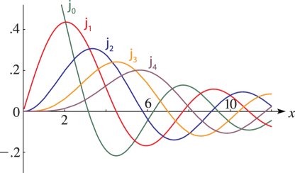
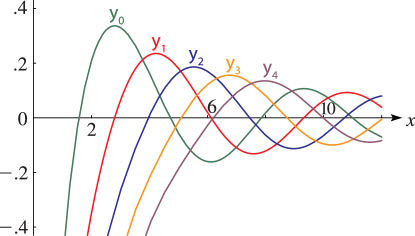
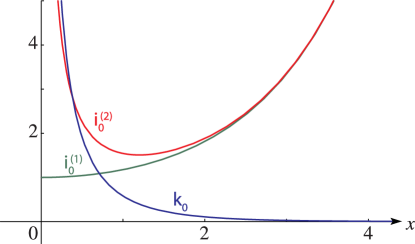
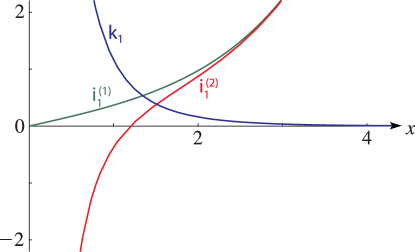
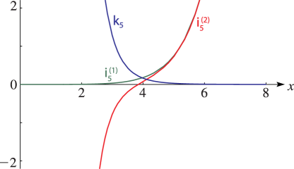
25: 10.48 Graphs

… ►

►►

Figure 10.48.1: ${𝗃}_n\left(x\right)$, $n=0(1)4$, $0\le x\le 12$. Magnify

►

►►

Figure 10.48.2: ${𝗒}_n\left(x\right)$, $n=0(1)4$, . Magnify

… ►

►►

Figure 10.48.5: ${𝗂}_0^{(1)}\left(x\right)$, ${𝗂}_0^{(2)}\left(x\right)$, ${𝗄}_0\left(x\right)$, $0\le x\le 4$. Magnify

►

►►

Figure 10.48.6: ${𝗂}_1^{(1)}\left(x\right),{𝗂}_1^{(2)}\left(x\right),{𝗄}_1\left(x\right)$, $0\le x\le 4$. Magnify

►

►►

Figure 10.48.7: ${𝗂}_5^{(1)}\left(x\right)$, ${𝗂}_5^{(2)}\left(x\right)$, ${𝗄}_5\left(x\right)$, $0\le x\le 8$. Magnify

26: 5.22 Tables

… ►Abramowitz and Stegun (1964, Chapter 6) tabulates $\mathrm{\Gamma }\left(x\right)$, $\ln \mathrm{\Gamma }\left(x\right)$, $\psi \left(x\right)$, and ${\psi }^{\prime }\left(x\right)$ for $x=1(.005)2$ to 10D; ${\psi }^{\prime \prime }\left(x\right)$ and ${\psi }^{(3)}\left(x\right)$ for $x=1(.01)2$ to 10D; $\mathrm{\Gamma }\left(n\right)$, $1/\mathrm{\Gamma }\left(n\right)$, $\mathrm{\Gamma }\left(n+\frac{1}{2}\right)$, $\psi \left(n\right)$, ${\log }_{10}\mathrm{\Gamma }\left(n\right)$, ${\log }_{10}\mathrm{\Gamma }\left(n+\frac{1}{3}\right)$, ${\log }_{10}\mathrm{\Gamma }\left(n+\frac{1}{2}\right)$, and ${\log }_{10}\mathrm{\Gamma }\left(n+\frac{2}{3}\right)$ for $n=1(1)101$ to 8–11S; $\mathrm{\Gamma }\left(n+1\right)$ for $n=100(100)1000$ to 20S. Zhang and Jin (1996, pp. 67–69 and 72) tabulates $\mathrm{\Gamma }\left(x\right)$, $1/\mathrm{\Gamma }\left(x\right)$, $\mathrm{\Gamma }\left(-x\right)$, $\ln \mathrm{\Gamma }\left(x\right)$, $\psi \left(x\right)$, $\psi \left(-x\right)$, ${\psi }^{\prime }\left(x\right)$, and ${\psi }^{\prime }\left(-x\right)$ for $x=0(.1)5$ to 8D or 8S; $\mathrm{\Gamma }\left(n+1\right)$ for $n=0(1)100(10)250(50)500(100)3000$ to 51S. … ►Abramov (1960) tabulates $\ln \mathrm{\Gamma }\left(x+\mathrm{i}y\right)$ for $x=1$ ($.01$) $2$, $y=0$ ($.01$) $4$ to 6D. Abramowitz and Stegun (1964, Chapter 6) tabulates $\ln \mathrm{\Gamma }\left(x+\mathrm{i}y\right)$ for $x=1$ ($.1$) $2$, $y=0$ ($.1$) $10$ to 12D. …Zhang and Jin (1996, pp. 70, 71, and 73) tabulates the real and imaginary parts of $\mathrm{\Gamma }\left(x+\mathrm{i}y\right)$, $\ln \mathrm{\Gamma }\left(x+\mathrm{i}y\right)$, and $\psi \left(x+\mathrm{i}y\right)$ for $x=0.5,1,5,10$, $y=0(.5)10$ to 8S.

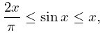
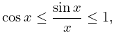
27: 4.18 Inequalities

… ►

4.18.1 $$\frac{2x}{\pi }\le \sin x\le x,$$ $0\le x\le \frac{1}{2}\pi$.

ⓘ

Symbols:

$\pi$: the ratio of the circumference of a circle to its diameter, $\sin z$: sine function and $x$: real variable

A&S Ref:

4.3.79 4.3.80

Referenced by:

§4.18

Permalink:

http://dlmf.nist.gov/4.18.E1

Encodings:

pMML, png, TeX

See also:

Annotations for §4.18, §4.18 and Ch.4

►

4.18.2 $$x\le \tan x,$$ ,

ⓘ

Symbols:

$\pi$: the ratio of the circumference of a circle to its diameter, $\tan z$: tangent function and $x$: real variable

A&S Ref:

4.3.80

Referenced by:

§4.18

Permalink:

http://dlmf.nist.gov/4.18.E2

Encodings:

pMML, png, TeX

See also:

Annotations for §4.18, §4.18 and Ch.4

►

4.18.3 $$\cos x\le \frac{\sin x}{x}\le 1,$$ $0\le x\le \pi$,

ⓘ

Symbols:

$\pi$: the ratio of the circumference of a circle to its diameter, $\cos z$: cosine function, $\sin z$: sine function and $x$: real variable

A&S Ref:

4.3.81

Referenced by:

§4.18

Permalink:

http://dlmf.nist.gov/4.18.E3

Encodings:

pMML, png, TeX

See also:

Annotations for §4.18, §4.18 and Ch.4

►

4.18.4 .

ⓘ

Symbols:

$\pi$: the ratio of the circumference of a circle to its diameter, $\sin z$: sine function and $x$: real variable

A&S Ref:

4.3.82

Referenced by:

§4.18

Permalink:

http://dlmf.nist.gov/4.18.E4

Encodings:

pMML, png, TeX

See also:

Annotations for §4.18, §4.18 and Ch.4

…

28: 26.1 Special Notation

… ►

$$x^{\overline{n}}=x(x+1)(x+2)\mathrm{\cdots }(x+n-1),$$

►

$$x^{\underset{¯}{n}}=x(x-1)(x-2)\mathrm{\cdots }(x-n+1).$$

…

29: 14.26 Uniform Asymptotic Expansions

… ►The uniform asymptotic approximations given in §14.15 for $P_{\nu }^{-\mu }\left(x\right)$ and ${𝑸}_{\nu }^{\mu }\left(x\right)$ for are extended to domains in the complex plane in the following references: §§14.15(i) and 14.15(ii), Dunster (2003b); §14.15(iii), Olver (1997b, Chapter 12); §14.15(iv), Boyd and Dunster (1986). …

30: 11.15 Approximations

… ►

Luke (1975, pp. 416–421) gives Chebyshev-series expansions for ${𝐇}_n\left(x\right)$, ${𝐋}_n\left(x\right)$, $0\le \left|x\right|\le 8$, and ${𝐇}_n\left(x\right)-Y_n\left(x\right)$, $x\ge 8$, for $n=0,1$; ${\int }_0^x{t}^{-m}{𝐇}_0\left(t\right)dt$, ${\int }_0^x{t}^{-m}{𝐋}_0\left(t\right)dt$, $0\le \left|x\right|\le 8$, $m=0,1$ and ${\int }_0^x({𝐇}_0\left(t\right)-Y_0\left(t\right))dt$, ${\int }_x^{\mathrm{\infty }}{t}^{-1}({𝐇}_0\left(t\right)-Y_0\left(t\right))dt$, $x\ge 8$; the coefficients are to 20D.

►

MacLeod (1993) gives Chebyshev-series expansions for ${𝐋}_0\left(x\right)$, ${𝐋}_1\left(x\right)$, $0\le x\le 16$, and $I_0\left(x\right)-{𝐋}_0\left(x\right)$, $I_1\left(x\right)-{𝐋}_1\left(x\right)$, $x\ge 16$; the coefficients are to 20D.

… ►

Newman (1984) gives polynomial approximations for ${𝐇}_n\left(x\right)$ for $n=0,1$, $0\le x\le 3$, and rational-fraction approximations for ${𝐇}_n\left(x\right)-Y_n\left(x\right)$ for $n=0,1$, $x\ge 3$. The maximum errors do not exceed 1.2×10⁻⁸ for the former and 2.5×10⁻⁸ for the latter.