as%20x%E2%86%92%C2%B11

SearchAdvancedHelp

(0.003 seconds)

21—30 of 687 matching pages

21: 23 Weierstrass Elliptic and Modular
Functions

…

22: 7.8 Inequalities

… ►Let $𝖬\left(x\right)$ denote Mills’ ratio: … ►

7.8.4 $x>-\frac{1}{2}\sqrt{2}$,

ⓘ

Symbols:

$𝖬\left(x\right)$: Mills’ ratio and $x$: real variable

Referenced by:

§7.8

Permalink:

http://dlmf.nist.gov/7.8.E4

Encodings:

pMML, png, TeX

See also:

Annotations for §7.8 and Ch.7

►

7.8.5 $x\ge 0$.

ⓘ

Symbols:

$𝖬\left(x\right)$: Mills’ ratio and $x$: real variable

Referenced by:

§7.8

Permalink:

http://dlmf.nist.gov/7.8.E5

Encodings:

pMML, png, TeX

See also:

Annotations for §7.8 and Ch.7

… ►The function $F\left(x\right)/\sqrt{1-{\mathrm{e}}^{-2x^2}}$ is strictly decreasing for $x>0$. For these and similar results for Dawson’s integral $F\left(x\right)$ see Janssen (2021). …

23: 10.3 Graphics

… ►For the modulus and phase functions $M_{\nu }\left(x\right)$, ${\theta }_{\nu }\left(x\right)$, $N_{\nu }\left(x\right)$, and ${\varphi }_{\nu }\left(x\right)$ see §10.18. ►

►►

Figure 10.3.1: $J_0\left(x\right)$, $Y_0\left(x\right)$, $J_1\left(x\right)$, $Y_1\left(x\right)$, $0\le x\le 10$. Magnify

►

►►

Figure 10.3.2: $J_5\left(x\right)$, $Y_5\left(x\right)$, $M_5\left(x\right)$, $0\le x\le 15$. Magnify

… ►

►

►

Figure 10.3.14: $H_5^{(1)}\left(x+\mathrm{i}y\right)$, $-20\le x\le 10$, $-4\le y\le 4$. … Magnify 3D Help

… ►

►

►

Figure 10.3.16: $H_{5.5}^{(1)}\left(x+\mathrm{i}y\right)$, $-20\le x\le 10$, $-4\le y\le 4$. … Magnify 3D Help

…

24: 22.3 Graphics

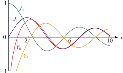
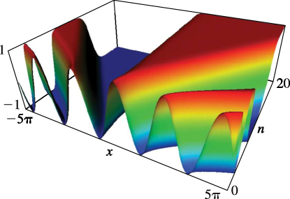
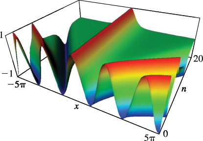
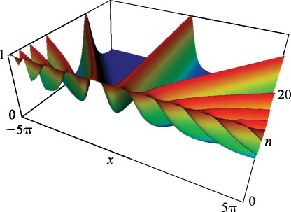
… ►Line graphs of the functions $\mathrm{sn}(x,k)$, $\mathrm{cn}(x,k)$, $\mathrm{dn}(x,k)$, $\mathrm{cd}(x,k)$, $\mathrm{sd}(x,k)$, $\mathrm{nd}(x,k)$, $\mathrm{dc}(x,k)$, $\mathrm{nc}(x,k)$, $\mathrm{sc}(x,k)$, $\mathrm{ns}(x,k)$, $\mathrm{ds}(x,k)$, and $\mathrm{cs}(x,k)$ for representative values of real $x$ and real $k$ illustrating the near trigonometric ($k=0$), and near hyperbolic ($k=1$) limits. 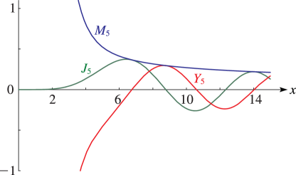… ► $\mathrm{sn}(x,k)$, $\mathrm{cn}(x,k)$, and $\mathrm{dn}(x,k)$ as functions of real arguments $x$ and $k$. … ►

►

►

Figure 22.3.13: $\mathrm{sn}(x,k)$ for $k=1-{\mathrm{e}}^{-n}$, $n=0$ to 20, $-5\pi \le x\le 5\pi$. Magnify 3D Help

►

►

►

Figure 22.3.14: $\mathrm{cn}(x,k)$ for $k=1-{\mathrm{e}}^{-n}$, $n=0$ to 20, $-5\pi \le x\le 5\pi$. Magnify 3D Help

►

►

►

Figure 22.3.15: $\mathrm{dn}(x,k)$ for $k=1-{\mathrm{e}}^{-n}$, $n=0$ to 20, $-5\pi \le x\le 5\pi$. Magnify 3D Help

…

25: 5.22 Tables

… ►Abramowitz and Stegun (1964, Chapter 6) tabulates $\mathrm{\Gamma }\left(x\right)$, $\ln \mathrm{\Gamma }\left(x\right)$, $\psi \left(x\right)$, and ${\psi }^{\prime }\left(x\right)$ for $x=1(.005)2$ to 10D; ${\psi }^{\prime \prime }\left(x\right)$ and ${\psi }^{(3)}\left(x\right)$ for $x=1(.01)2$ to 10D; $\mathrm{\Gamma }\left(n\right)$, $1/\mathrm{\Gamma }\left(n\right)$, $\mathrm{\Gamma }\left(n+\frac{1}{2}\right)$, $\psi \left(n\right)$, ${\log }_{10}\mathrm{\Gamma }\left(n\right)$, ${\log }_{10}\mathrm{\Gamma }\left(n+\frac{1}{3}\right)$, ${\log }_{10}\mathrm{\Gamma }\left(n+\frac{1}{2}\right)$, and ${\log }_{10}\mathrm{\Gamma }\left(n+\frac{2}{3}\right)$ for $n=1(1)101$ to 8–11S; $\mathrm{\Gamma }\left(n+1\right)$ for $n=100(100)1000$ to 20S. Zhang and Jin (1996, pp. 67–69 and 72) tabulates $\mathrm{\Gamma }\left(x\right)$, $1/\mathrm{\Gamma }\left(x\right)$, $\mathrm{\Gamma }\left(-x\right)$, $\ln \mathrm{\Gamma }\left(x\right)$, $\psi \left(x\right)$, $\psi \left(-x\right)$, ${\psi }^{\prime }\left(x\right)$, and ${\psi }^{\prime }\left(-x\right)$ for $x=0(.1)5$ to 8D or 8S; $\mathrm{\Gamma }\left(n+1\right)$ for $n=0(1)100(10)250(50)500(100)3000$ to 51S. … ►Abramov (1960) tabulates $\ln \mathrm{\Gamma }\left(x+\mathrm{i}y\right)$ for $x=1$ ($.01$) $2$, $y=0$ ($.01$) $4$ to 6D. …This reference also includes $\psi \left(x+\mathrm{i}y\right)$ for the same arguments to 5D. Zhang and Jin (1996, pp. 70, 71, and 73) tabulates the real and imaginary parts of $\mathrm{\Gamma }\left(x+\mathrm{i}y\right)$, $\ln \mathrm{\Gamma }\left(x+\mathrm{i}y\right)$, and $\psi \left(x+\mathrm{i}y\right)$ for $x=0.5,1,5,10$, $y=0(.5)10$ to 8S.

26: 36.5 Stokes Sets

… ►The Stokes set consists of the rays $\mathrm{ph}x=\pm 2\pi /3$ in the complex $x$-plane. … ►where $x_{\pm }$ are the two smallest positive roots of the equation … ►The first sheet corresponds to and is generated as a solution of Equations (36.5.6)–(36.5.9). … ►When $|X|>X_2$ the Stokes set $Y_{\mathrm{S}}(X)$ is given by … ►Alternatively, when …

27: Bibliography N

… ►

On an integral transform involving a class of Mathieu functions. SIAM J. Math. Anal. 20 (6), pp. 1500–1513.

ⓘ

External Links:

ISSN 0036-1410, Document, MathReview (K. C. Gupta), ZentralBlatt

Referenced by:

§28.26(ii).

Encodings:

BibTeX

… ►

Reduction and evaluation of elliptic integrals. Math. Comp. 20 (94), pp. 223–231.

ⓘ

External Links:

FullText, MathReview (I. A. Stegun), ZentralBlatt

Referenced by:

§19.37(iv).

Encodings:

BibTeX

… ►

The resurgence properties of the incomplete gamma function II. Stud. Appl. Math. 135 (1), pp. 86–116.

ⓘ

External Links:

ISSN 0022-2526, Document, Link, MathReview Entry, ZentralBlatt

Referenced by:

§8.11(iii).

Encodings:

BibTeX

… ►

A table of integrals of the error functions. J. Res. Nat. Bur. Standards Sect B. 73B, pp. 1–20.

ⓘ

Notes:

See for additions and corrections same journal, Sect. B 75, 149–163 (1975)

External Links:

MathReview, ZentralBlatt

Referenced by:

§7.14(iii), §7.21, §7.7(iii).

Encodings:

BibTeX

… ►

Symmetries in the fourth Painlevé equation and Okamoto polynomials. Nagoya Math. J. 153, pp. 53–86.

ⓘ

External Links:

ISSN 0027-7630, MathReview (Andrei A. Kapaev), ZentralBlatt

Referenced by:

§32.8(iv).

Encodings:

BibTeX

…

28: 3.4 Differentiation

… ►If $f^{(n+2)}(x)$ is continuous on the interval $I$ defined in §3.3(i), then the remainder in (3.4.1) is given by … ►where $C$ is a simple closed contour described in the positive rotational sense such that $C$ and its interior lie in the domain of analyticity of $f$, and $x_0$ is interior to $C$. Taking $C$ to be a circle of radius $r$ centered at $x_0$, we obtain … ► $f(z)={\mathrm{e}}^z$, $x_0=0$. … ►For partial derivatives we use the notation $u_{t,s}=u(x_0+th,y_0+sh)$. …

29: 7.23 Tables

… ►

Abramowitz and Stegun (1964, Chapter 7) includes $\mathrm{erf}x$, $(2/\sqrt{\pi }){\mathrm{e}}^{-x^2}$, $x\in [0,2]$, 10D; $(2/\sqrt{\pi }){\mathrm{e}}^{-x^2}$, $x\in [2,10]$, 8S; $x{\mathrm{e}}^{x^2}\mathrm{erfc}x$, $x^{-2}\in [0,0.25]$, 7D; $2^n\mathrm{\Gamma }\left(\frac{1}{2}n+1\right){\mathrm{i}}^n\mathrm{erfc}\left(x\right)$, $n=1(1)6,10,11$, $x\in [0,5]$, 6S; $F\left(x\right)$, $x\in [0,2]$, 10D; $xF\left(x\right)$, $x^{-2}\in [0,0.25]$, 9D; $C\left(x\right)$, $S\left(x\right)$, $x\in [0,5]$, 7D; $\mathrm{f}\left(x\right)$, $\mathrm{g}\left(x\right)$, $x\in [0,1]$, $x^{-1}\in [0,1]$, 15D.

►

Abramowitz and Stegun (1964, Table 27.6) includes the Goodwin–Staton integral $G\left(x\right)$, $x=1(.1)3(.5)8$, 4D; also $G\left(x\right)+\ln x$, $x=0(.05)1$, 4D.

… ►

Zhang and Jin (1996, pp. 637, 639) includes $(2/\sqrt{\pi }){\mathrm{e}}^{-x^2}$, $\mathrm{erf}x$, $x=0(.02)1(.04)3$, 8D; $C\left(x\right)$, $S\left(x\right)$, $x=0(.2)10(2)100(100)500$, 8D.

►

§7.23(iii) Complex Variables, $z=x+\mathrm{i}y$

… ►

Zhang and Jin (1996, pp. 638, 640–641) includes the real and imaginary parts of $\mathrm{erf}z$, $x\in [0,5]$, $y=0.5(.5)3$, 7D and 8D, respectively; the real and imaginary parts of ${\int }_x^{\mathrm{\infty }}{\mathrm{e}}^{\pm \mathrm{i}{t}^2}dt$, $(1/\sqrt{\pi }){\mathrm{e}}^{\mp \mathrm{i}(x^2+(\pi /4))}{\int }_x^{\mathrm{\infty }}{\mathrm{e}}^{\pm \mathrm{i}{t}^2}dt$, $x=0(.5)20(1)25$, 8D, together with the corresponding modulus and phase to 8D and 6D (degrees), respectively.

…

30: 36 Integrals with Coalescing Saddles

…