analytic continuation onto higher Riemann sheets
(0.003 seconds)
1—10 of 273 matching pages
1: 21.7 Riemann Surfaces
§21.7 Riemann Surfaces
►§21.7(i) Connection of Riemann Theta Functions to Riemann Surfaces
… ►Removing the singularities of this curve gives rise to a two-dimensional connected manifold with a complex-analytic structure, that is, a Riemann surface. All compact Riemann surfaces can be obtained this way. ►Since a Riemann surface is a two-dimensional manifold that is orientable (owing to its analytic structure), its only topological invariant is its genus (the number of handles in the surface). … ►where , are analytic functions. …2: 25.1 Special Notation
…
►
►
►The main function treated in this chapter is the Riemann zeta function .
This notation was introduced in Riemann (1859).
►The main related functions are the Hurwitz zeta function , the dilogarithm , the polylogarithm (also known as Jonquière’s function ), Lerch’s transcendent , and the Dirichlet -functions .
| nonnegative integers. | |
| … | |
3: 21.2 Definitions
…
►
§21.2(i) Riemann Theta Functions
… ►This -tuple Fourier series converges absolutely and uniformly on compact sets of the and spaces; hence is an analytic function of (each element of) and (each element of) . … ►For numerical purposes we use the scaled Riemann theta function , defined by (Deconinck et al. (2004)), …Many applications involve quotients of Riemann theta functions: the exponential factor then disappears. … ►§21.2(ii) Riemann Theta Functions with Characteristics
…4: 15.17 Mathematical Applications
…
►The quotient of two solutions of (15.10.1) maps the closed upper half-plane conformally onto a curvilinear triangle.
…
►The three singular points in Riemann’s differential equation (15.11.1) lead to an interesting Riemann sheet structure.
By considering, as a group, all analytic transformations of a basis of solutions under analytic continuation around all paths on the Riemann sheet, we obtain the monodromy group.
These monodromy groups are finite iff the solutions of Riemann’s differential equation are all algebraic.
…
5: 1.18 Linear Second Order Differential Operators and Eigenfunction Expansions
…
►Note that the integral in (1.18.66) is not singular if approached separately from above, or below, the real axis: in fact analytic continuation from the upper half of the complex plane, across the cut, and onto higher Riemann Sheets can access complex poles with singularities at discrete energies corresponding to quantum resonances, or decaying quantum states with lifetimes proportional to .
For this latter see Simon (1973), and Reinhardt (1982); wherein advantage is taken of the fact that although branch points are actual singularities of an analytic function, the location of the branch cuts are often at our disposal, as they are not singularities of the function, but simply arbitrary lines to keep a function single valued, and thus only singularities of a specific representation of that analytic function.
This is accomplished by the variable change , in , which rotates the continuous spectrum and the branch cut of (1.18.66) into the lower half complex plain by the angle , with respect to the unmoved branch point at ; thus, providing access to resonances on the higher Riemann sheet should be large enough to expose them.
This dilatation transformation, which does require analyticity of in (1.18.28), or an analytic approximation thereto, leaves the poles, corresponding to the discrete spectrum, invariant, as they are, as is the branch point, actual singularities of .
…
6: 6.4 Analytic Continuation
§6.4 Analytic Continuation
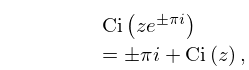
►Analytic continuation of the principal value of yields a multi-valued function with branch points at and . … ►
6.4.4
…
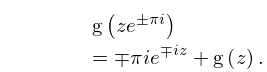
►
6.4.7
…
7: 28.7 Analytic Continuation of Eigenvalues
§28.7 Analytic Continuation of Eigenvalues
►As functions of , and can be continued analytically in the complex -plane. … ►All the , , can be regarded as belonging to a complete analytic function (in the large). … ►
28.7.4
8: 1.10 Functions of a Complex Variable
…
►
§1.10(ii) Analytic Continuation
… ►Analytic continuation is a powerful aid in establishing transformations or functional equations for complex variables, because it enables the problem to be reduced to: (a) deriving the transformation (or functional equation) with real variables; followed by (b) finding the domain on which the transformed function is analytic. ►Schwarz Reflection Principle
… ►Analytic Functions
… ►Then the value of at any other point is obtained by analytic continuation. …9: 18.40 Methods of Computation
…
►
