Stokes%20phenomenon

SearchAdvancedHelp

(0.002 seconds)

1—10 of 112 matching pages

1: 36.5 Stokes Sets

§36.5 Stokes Sets

►

§36.5(i) Definitions

… ►

§36.5(ii) Cuspoids

… ►

Elliptic Umbilic Stokes Set (Codimension three)

… ►

§36.5(iv) Visualizations

…

2: Bibliography P

… ►

Stokes phenomenon demystified. Bull. Inst. Math. Appl. 31 (1-2), pp. 21–28.

ⓘ

External Links:

ISSN 0905-5628, MathReview Entry, ZentralBlatt

Referenced by:

§2.11(iv).

Encodings:

BibTeX

… ►

Smoothing of the Stokes phenomenon for high-order differential equations. Proc. Roy. Soc. London Ser. A 436, pp. 165–186.

ⓘ

External Links:

ISSN 0962-8444, FullText, MathReview (F. W. J. Olver), ZentralBlatt

Referenced by:

§2.11(v).

Encodings:

BibTeX

►

Smoothing of the Stokes phenomenon using Mellin-Barnes integrals. J. Comput. Appl. Math. 41 (1-2), pp. 117–133.

ⓘ

External Links:

ISSN 0377-0427, Document, MathReview (Anatoly Kilbas), ZentralBlatt

Referenced by:

§2.11(v).

Encodings:

BibTeX

… ►

The Stokes phenomenon associated with the Hurwitz zeta function $\zeta (s,a)$ . Proc. Roy. Soc. London Ser. A 461, pp. 297–304.

ⓘ

External Links:

ISSN 1364-5021, Document, MathReview (Marc Prevost), ZentralBlatt

Referenced by:

(25.11.43), §25.11(xii).

Encodings:

BibTeX

… ►

Automatic computation of Bessel function integrals. Comput. Phys. Comm. 25 (3), pp. 289–295.

ⓘ

Notes:

Double-precision Fortran, maximum accuracy 20S.

External Links:

ISSN 0010-4655, Document, Code

Referenced by:

6th item.

Encodings:

BibTeX

…

3: 2.11 Remainder Terms; Stokes Phenomenon

§2.11 Remainder Terms; Stokes Phenomenon

… ►

§2.11(iv) Stokes Phenomenon

… ►That the change in their forms is discontinuous, even though the function being approximated is analytic, is an example of the Stokes phenomenon. Where should the change-over take place? Can it be accomplished smoothly? … ►For higher-order Stokes phenomena see Olde Daalhuis (2004b) and Howls et al. (2004). …

4: 7.20 Mathematical Applications

… ►For applications of the complementary error function in uniform asymptotic approximations of integrals—saddle point coalescing with a pole or saddle point coalescing with an endpoint—see Wong (1989, Chapter 7), Olver (1997b, Chapter 9), and van der Waerden (1951). ►The complementary error function also plays a ubiquitous role in constructing exponentially-improved asymptotic expansions and providing a smooth interpretation of the Stokes phenomenon; see §§2.11(iii) and 2.11(iv). …

5: 8.22 Mathematical Applications

… ►

8.22.1 $$F_p\left(z\right)=\frac{\mathrm{\Gamma }\left(p\right)}{2\pi }{z}^{1-p}{E}_p\left(z\right)=\frac{\mathrm{\Gamma }\left(p\right)}{2\pi }\mathrm{\Gamma }(1-p,z),$$

ⓘ

Symbols:

$\mathrm{\Gamma }\left(z\right)$: gamma function, $\pi$: the ratio of the circumference of a circle to its diameter, $E_p\left(z\right)$: generalized exponential integral, $\mathrm{\Gamma }(a,z)$: incomplete gamma function, $F_p\left(z\right)$: terminant function, $z$: complex variable and $p$: parameter

Permalink:

http://dlmf.nist.gov/8.22.E1

Encodings:

pMML, png, TeX

See also:

Annotations for §8.22(i), §8.22 and Ch.8

►plays a fundamental role in re-expansions of remainder terms in asymptotic expansions, including exponentially-improved expansions and a smooth interpretation of the Stokes phenomenon. …

6: Bibliography I

… ►

The real roots of Bernoulli polynomials. Ann. Univ. Turku. Ser. A I 37, pp. 1–20.

ⓘ

External Links:

MathReview (D. H. Lehmer), ZentralBlatt

Referenced by:

§24.12(i).

Encodings:

BibTeX

… ►

Quasi-linear Stokes phenomenon for the second Painlevé transcendent. Nonlinearity 16 (1), pp. 363–386.

ⓘ

External Links:

ISSN 0951-7715, Document, MathReview (Youmin Lu), ZentralBlatt

Referenced by:

§32.12(ii).

Encodings:

BibTeX

…

7: 10.46 Generalized and Incomplete Bessel Functions; Mittag-Leffler Function

… ►For exponentially-improved asymptotic expansions in the same circumstances, together with smooth interpretations of the corresponding Stokes phenomenon (§§2.11(iii)–2.11(v)) see Wong and Zhao (1999b) when $\rho >0$, and Wong and Zhao (1999a) when . … ►This reference includes exponentially-improved asymptotic expansions for $E_{a,b}\left(z\right)$ when $|z|\to \mathrm{\infty }$, together with a smooth interpretation of Stokes phenomena. …

8: Bibliography K

… ►

Essential singularity of the Painlevé function of the second kind and the nonlinear Stokes phenomenon. Zap. Nauchn. Sem. Leningrad. Otdel. Mat. Inst. Steklov. (LOMI) 187, pp. 139–170 (Russian).

ⓘ

Notes:

English translation: J. Math. Sci. 73(1995), no. 4, pp. 500–517

External Links:

ISSN 0373-2703, Document, MathReview (Andreĭ Bolibrukh), ZentralBlatt

Referenced by:

§32.12(ii).

Encodings:

BibTeX

►

Quasi-linear Stokes phenomenon for the Painlevé first equation. J. Phys. A 37 (46), pp. 11149–11167.

ⓘ

External Links:

ISSN 0305-4470, Document, MathReview (W. Balser), ZentralBlatt

Referenced by:

§32.12(i).

Encodings:

BibTeX

… ►

Algorithm 737: INTLIB: A portable Fortran 77 interval standard-function library. ACM Trans. Math. Software 20 (4), pp. 447–459.

ⓘ

External Links:

ISSN 0098-3500, Document, GAMS (module 737; package TOMS), ZentralBlatt

Referenced by:

1st item.

Encodings:

BibTeX

… ►

Methods of computing the Riemann zeta-function and some generalizations of it. USSR Comput. Math. and Math. Phys. 20 (6), pp. 212–230.

ⓘ

External Links:

Document, MathReview (Matti Jutila), ZentralBlatt

Referenced by:

§25.18(i).

Encodings:

BibTeX

… ►

Connection formulae for asymptotics of solutions of the degenerate third Painlevé equation. I. Inverse Problems 20 (4), pp. 1165–1206.

ⓘ

External Links:

ISSN 0266-5611, Document, MathReview (Shun Shimomura), ZentralBlatt

Referenced by:

§32.11(iv).

Encodings:

BibTeX

…

9: 6.16 Mathematical Applications

… ►

§6.16(i) The Gibbs Phenomenon

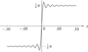
… ►This nonuniformity of convergence is an illustration of the Gibbs phenomenon. … ►

►►

Figure 6.16.1: Graph of $S_n(x)$, $n=250$, $-0.1\le x\le 0.1$, illustrating the Gibbs phenomenon. Magnify

… ►

►►

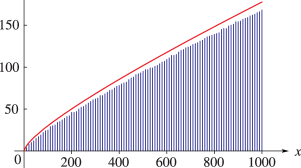
Figure 6.16.2: The logarithmic integral $\mathrm{li}\left(x\right)$, together with vertical bars indicating the value of $\pi (x)$ for $x=10,20,\mathrm{\dots },1000$. Magnify

10: Bibliography B

… ►

Stokes surfaces of diffraction catastrophes with codimension three. Nonlinearity 3 (2), pp. 281–291.

ⓘ

External Links:

ISSN 0951-7715, Document, MathReview (Maria Carmen Romero-Fuster), ZentralBlatt

Referenced by:

§36.2(i), §36.5(ii), §36.5(iii), §36.5(iv).

Encodings:

BibTeX

… ►

Overlapping Stokes smoothings: Survival of the error function and canonical catastrophe integrals. Proc. Roy. Soc. London Ser. A 444, pp. 201–216.

ⓘ

External Links:

ISSN 0962-8444, FullText, MathReview (F. Ursell), ZentralBlatt

Referenced by:

§36.12(iii).

Encodings:

BibTeX

… ►

Uniform asymptotic smoothing of Stokes’s discontinuities. Proc. Roy. Soc. London Ser. A 422, pp. 7–21.

ⓘ

External Links:

ISSN 0080-4630, FullText, MathReview (André Hautot), ZentralBlatt

Referenced by:

§2.11(iv).

Encodings:

BibTeX

►

Infinitely many Stokes smoothings in the gamma function. Proc. Roy. Soc. London Ser. A 434, pp. 465–472.

ⓘ

External Links:

ISSN 0962-8444, FullText, MathReview (E. Riekstiņš), ZentralBlatt

Referenced by:

§5.11(ii).

Encodings:

BibTeX

… ►

Stieltjes transforms and the Stokes phenomenon. Proc. Roy. Soc. London Ser. A 429, pp. 227–246.

ⓘ

External Links:

ISSN 0962-8444, FullText, MathReview, ZentralBlatt

Referenced by:

§2.11(v).

Encodings:

BibTeX

…