SL(2,Z)
(0.003 seconds)
21—30 of 803 matching pages
21: 22.1 Special Notation
…
►
►
…
►The functions treated in this chapter are the three principal Jacobian elliptic functions , , ; the nine subsidiary Jacobian elliptic functions , , , , , , , , ; the amplitude function ; Jacobi’s epsilon and zeta functions and .
…
►Other notations for are and with ; see Abramowitz and Stegun (1964) and Walker (1996).
…
| real variables. | |
| … | |
| complementary modulus, . If , then . | |
| … | |
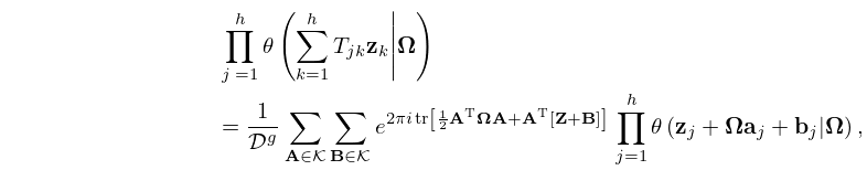
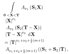
22: 21.6 Products
…
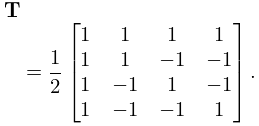
►Also, let be an arbitrary matrix.
…
►
21.6.3
►where , , denote respectively the th columns of , , .
…
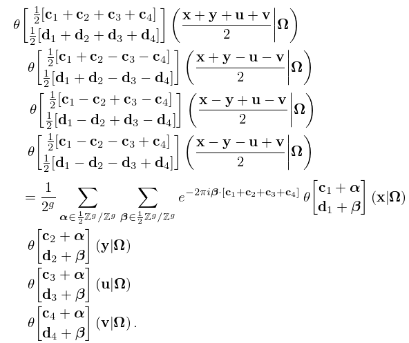
►
21.6.5
…
►
21.6.7
…
23: 18.8 Differential Equations
24: 18.40 Methods of Computation
…
►Results of low ( to decimal digits) precision for are easily obtained for to .
…
►Convergence is .
…
►Here is an interpolation of the abscissas , that is, , allowing differentiation by .
…where the coefficients are defined recursively via , and
…The PWCF is a minimally oscillatory algebraic interpolation of the abscissas .
…
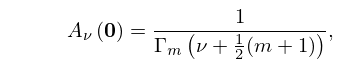
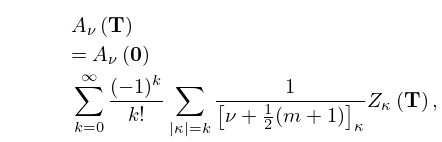
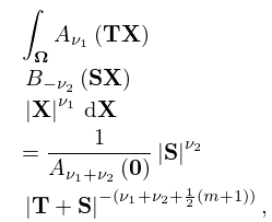
25: 35.5 Bessel Functions of Matrix Argument
26: Bibliography E
…
►
Interlacing properties of the zeros of Bessel functions.
Atti Sem. Mat. Fis. Univ. Modena XLII (2), pp. 525–529.
►
An upper bound for the zeros of the derivative of Bessel functions.
Rend. Circ. Mat. Palermo (2) 46 (1), pp. 123–130.
…
►
A formula including Legendre’s
.
Messenger of Math. 33, pp. 31–32.
…
►
Painlevé transcendent describes quantum correlation function of the antiferromagnet away from the free-fermion point.
J. Phys. A 29 (17), pp. 5619–5626.
…
►
On the transformation theory of ordinary second-order linear symmetric differential expressions.
Czechoslovak Math. J. 32(107) (2), pp. 275–306.
…
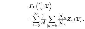
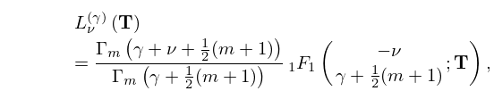
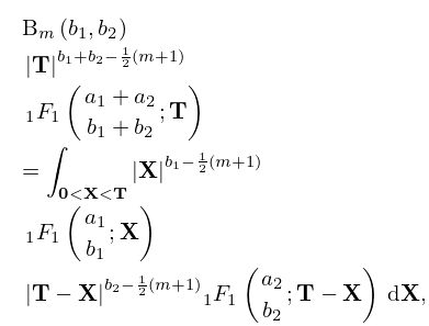
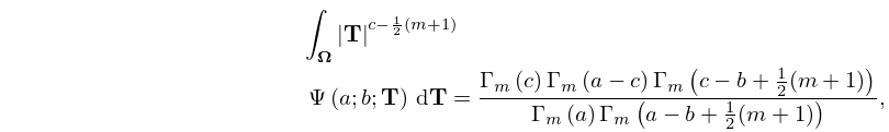
27: 35.6 Confluent Hypergeometric Functions of Matrix Argument
28: Bibliography P
…
►
A Kummer-type transformation for a hypergeometric function.
J. Comput. Appl. Math. 173 (2), pp. 379–382.
…
►
Optical properties of layer antiferromagnets with structure.
J. Phys. C: Solid State Physics 2 (11), pp. 2012–2021.
►
Complex zeros of the modified Bessel function
.
Math. Comp. 26 (120), pp. 949–953.
…
►
Numerical calculation of the generalized Fermi-Dirac integrals.
Comput. Phys. Comm. 55 (2), pp. 127–136.
…
►
Recurrence formulas for Coulomb wave functions.
Physical Rev. (2) 72 (7), pp. 626–627.
…
29: 9.13 Generalized Airy Functions
…
►and is any linear combination of the modified Bessel functions and (§10.25(ii)).
…
►The function on the right-hand side is recessive in the sector , and is therefore an essential member of any numerically satisfactory pair of solutions in this region.
…
►where and .
…
►The integration paths , , , are depicted in Figure 9.13.1.
, , are depicted in Figure 9.13.2.
…
