OP%E2%80%99s

SearchAdvancedHelp

(0.002 seconds)

21—30 of 609 matching pages

21: 18.33 Polynomials Orthogonal on the Unit Circle

… ►Simon (2005a, b) gives the general theory of these OP’s in terms of monic OP’s ${\mathrm{\Phi }}_n(x)$, see §18.33(vi). … ►

§18.33(iii) Connection with OP’s on the Line

… ►Let $\{p_n(x)\}$ and $\{q_n(x)\}$, $n=0,1,\mathrm{\dots }$, be OP’s with weight functions $w_1(x)$ and $w_2(x)$, respectively, on $(-1,1)$. … ►Instead of (18.33.9) one might take monic OP’s $\{q_n(x)\}$ with weight function $(1+x)w_1(x)$, and then express $q_n\left(\frac{1}{2}(z+z^{-1})\right)$ in terms of ${\varphi }_{2n}(z^{\pm 1})$ or ${\varphi }_{2n+1}(z^{\pm 1})$. After a quadratic transformation (18.2.23) this would express OP’s on $[-1,1]$ with an even orthogonality measure in terms of the ${\varphi }_n$. …

22: 18.30 Associated OP’s

§18.30 Associated OP’s

… ►

§18.30(vi) Corecursive Orthogonal Polynomials

… ►Note that this is the same recurrence as in (18.2.8) for the traditional OP’s, but with a different initialization. … ►

Associated Monic OP’s

… ►

Relationship of Monic Corecursive and Monic Associated OP’s

…

23: 18.9 Recurrence Relations and Derivatives

… ►For the other classical OP’s see Table 18.9.1; compare also §18.2(iv). … ►For the other classical OP’s see Table 18.9.2. … ►For the monic versions of the classical OP’s the recurrence coefficients $b_n$ and $c_n$ (there written as ${\alpha }_n$ and ${\beta }_n$, respectively) are given in §3.5(vi). They imply the recurrence coefficients for the orthonormal versions of the classical OP’s as well, see again §3.5(vi). … ►The following three formulas change the degree but preserve the parameters, see (18.2.42)–(18.2.44) for similar formulas for more general OP’s. …

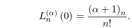
24: 18.6 Symmetry, Special Values, and Limits to Monomials

… ►

18.6.1 $$L_n^{(\alpha )}\left(0\right)=\frac{{\left(\alpha +1\right)}_n}{n!}.$$

ⓘ

Symbols:

$L_n^{(\alpha )}\left(x\right)$: Laguerre (or generalized Laguerre) polynomial, ${\left(a\right)}_n$: Pochhammer’s symbol (or shifted factorial), $!$: factorial (as in $n!$) and $n$: nonnegative integer

A&S Ref:

22.4.7 (see column for $f_n(0)$)

Referenced by:

§18.17(i), §18.6(i), §18.6(ii)

Permalink:

http://dlmf.nist.gov/18.6.E1

Encodings:

pMML, png, TeX

See also:

Annotations for §18.6(i), §18.6(i), §18.6 and Ch.18

►

Table 18.6.1: Classical OP’s: symmetry and special values.

► ►►

$p_n(x)$	$p_n(-x)$	$p_n(1)$	$p_{2n}(0)$	$p_{2n+1}^{\prime }(0)$
…

►

…

25: DLMF Project News

error generating summary

26: 18.27 $q$-Hahn Class

… ►The $q$-hypergeometric OP’s comprise the $q$-Hahn class (or $q$-linear lattice class) OP’s and the Askey–Wilson class (or $q$-quadratic lattice class) OP’s (§18.28). … ►A (nonexhaustive) classification of such systems of OP’s was made by Hahn (1949). There are 18 families of OP’s of $q$-Hahn class. … ►All these systems of OP’s have orthogonality properties of the form …Some of the systems of OP’s that occur in the classification do not have a unique orthogonality property. …

27: 18.20 Hahn Class: Explicit Representations

… ►

Table 18.20.1: Krawtchouk, Meixner, and Charlier OP’s: Rodrigues formulas (18.20.1).

► ►►

$p_n(x)$	$F(x)$	${\kappa }_n$
…

►

… ►

18.20.9 $$p_n(x;a,b,\overline{a},\overline{b})=\frac{{\mathrm{i}}^n{\left(a+\overline{a}\right)}_n{\left(a+\overline{b}\right)}_n}{n!}{}_3{}^{}F_2^{}(\genfrac{}{}{0pt}{}{-n,n+2\mathrm{\Re }\left(a+b\right)-1,a+\mathrm{i}x}{a+\overline{a},a+\overline{b}};1).$$

ⓘ

Symbols:

${}_p{}^{}F_q^{}(a_1,\mathrm{\dots },a_p;b_1,\mathrm{\dots },b_q;z)$ or ${}_p{}^{}F_q^{}(\genfrac{}{}{0pt}{}{a_1,\mathrm{\dots },a_p}{b_1,\mathrm{\dots },b_q};z)$: alternatively ${}_p{}^{}F_q^{}(𝐚;𝐛;z)$ or ${}_p{}^{}F_q^{}(\genfrac{}{}{0pt}{}{𝐚}{𝐛};z)$
generalized hypergeometric function, ${\left(a\right)}_n$: Pochhammer’s symbol (or shifted factorial), $\overline{z}$: complex conjugate, $p_n(x;a,b,\overline{a},\overline{b})$: continuous Hahn polynomial, $!$: factorial (as in $n!$), $\mathrm{i}$: imaginary unit, $\mathrm{\Re }$: real part, $n$: nonnegative integer and $x$: real variable

Referenced by:

§18.19, §18.20(ii), §18.21(ii), §18.22(iii), §18.26(ii)

Permalink:

http://dlmf.nist.gov/18.20.E9

Encodings:

pMML, png, TeX

See also:

Annotations for §18.20(ii), §18.20 and Ch.18

… ►

18.20.10 $$P_n^{(\lambda )}(x;\varphi )=\frac{{\left(2\lambda \right)}_n}{n!}{\mathrm{e}}^{\mathrm{i}n\varphi }{}_2{}^{}F_1^{}(\genfrac{}{}{0pt}{}{-n,\lambda +\mathrm{i}x}{2\lambda };1-{\mathrm{e}}^{-2\mathrm{i}\varphi }).$$

ⓘ

Symbols:

${}_2{}^{}F_1^{}(a,b;c;z)$: $=F(a,b;c;z)$ notation for Gauss’ hypergeometric function, $P_n^{(\lambda )}(x;\varphi )$: Meixner–Pollaczek polynomial, ${\left(a\right)}_n$: Pochhammer’s symbol (or shifted factorial), $\mathrm{e}$: base of natural logarithm, $!$: factorial (as in $n!$), $\mathrm{i}$: imaginary unit, $n$: nonnegative integer and $x$: real variable

Referenced by:

§18.19, §18.20(ii), §18.21(ii), §18.22(iii), §18.26(ii), (18.35.9)

Permalink:

http://dlmf.nist.gov/18.20.E10

Encodings:

pMML, png, TeX

See also:

Annotations for §18.20(ii), §18.20 and Ch.18

28: 18.5 Explicit Representations

… ►

18.5.5 $$p_n(x)=\frac{1}{{\kappa }_{n}w(x)}\frac{d^n}{{dx}^n}\left(w(x){(F(x))}^n\right).$$

ⓘ

Symbols:

$\frac{df}{dx}$: derivative of $f$ with respect to $x$ , $p_n(x)$: polynomial of degree $n$ , $w(x)$: weight function, $n$: nonnegative integer and $x$: real variable

A&S Ref:

22.1.6 (incorrectly stated as property of general OP’s)

Referenced by:

§18.17(v), §18.17(vi), §18.17(vii), item 3., §18.39(ii), §18.39(ii), Table 18.5.1, §18.9(iii)

Permalink:

http://dlmf.nist.gov/18.5.E5

Encodings:

pMML, png, TeX

See also:

Annotations for §18.5(ii), §18.5 and Ch.18

… ►

Table 18.5.1: Classical OP’s: Rodrigues formulas (18.5.5).

► ►►

$p_n(x)$	$w(x)$	$F(x)$	${\kappa }_n$
…

►

… ►

18.5.9 $$C_n^{(\lambda )}\left(x\right)=\frac{{\left(2\lambda \right)}_n}{n!}{}_2{}^{}F_1^{}(\genfrac{}{}{0pt}{}{-n,n+2\lambda }{\lambda +\frac{1}{2}};\frac{1-x}{2}),$$

ⓘ

Symbols:

${}_2{}^{}F_1^{}(a,b;c;z)$: $=F(a,b;c;z)$ notation for Gauss’ hypergeometric function, ${\left(a\right)}_n$: Pochhammer’s symbol (or shifted factorial), $!$: factorial (as in $n!$), $C_n^{(\lambda )}\left(x\right)$: ultraspherical (or Gegenbauer) polynomial, $n$: nonnegative integer and $x$: real variable

A&S Ref:

22.5.46

Referenced by:

§18.5(iii), §18.6(i)

Permalink:

http://dlmf.nist.gov/18.5.E9

Encodings:

pMML, png, TeX

See also:

Annotations for §18.5(iii), §18.5(iii), §18.5 and Ch.18

… ►

18.5.12 $$L_n^{(\alpha )}\left(x\right)=\sum _{\mathrm{\ell }=0}^n\frac{{\left(\alpha +\mathrm{\ell }+1\right)}_{n-\mathrm{\ell }}}{(n-\mathrm{\ell })!\mathrm{\ell }!}{(-x)}^{\mathrm{\ell }}=\frac{{\left(\alpha +1\right)}_n}{n!}{}_1{}^{}F_1^{}(\genfrac{}{}{0pt}{}{-n}{\alpha +1};x).$$

ⓘ

Symbols:

${}_1{}^{}F_1^{}(a;b;z)$: $=M(a,b,z)$ notation for the Kummer confluent hypergeometric function, $L_n^{(\alpha )}\left(x\right)$: Laguerre (or generalized Laguerre) polynomial, ${\left(a\right)}_n$: Pochhammer’s symbol (or shifted factorial), $!$: factorial (as in $n!$), $\mathrm{\ell }$: nonnegative integer, $n$: nonnegative integer and $x$: real variable

A&S Ref:

22.5.54

Referenced by:

§18.11(i), §18.17(v), §18.17(vi), §18.17(vii), §18.18(iii), §18.21(ii), Table 18.3.1, (18.34.1), §18.34(i), §18.5(iii), §18.6(ii)

Permalink:

http://dlmf.nist.gov/18.5.E12

Encodings:

pMML, png, TeX

See also:

Annotations for §18.5(iii), §18.5(iii), §18.5 and Ch.18

… ►

$U_6\left(x\right)=64x^6-80x^4+24x^2-1.$

…

29: 18.28 Askey–Wilson Class

… ►The Askey–Wilson class OP’s comprise the four-parameter families of Askey–Wilson polynomials and of $q$-Racah polynomials, and cases of these families obtained by specialization of parameters. The Askey–Wilson polynomials form a system of OP’s $\{p_n(x)\}$, $n=0,1,2,\mathrm{\dots }$, that are orthogonal with respect to a weight function on a bounded interval, possibly supplemented with discrete weights on a finite set. … ►In the remainder of this section the Askey–Wilson class OP’s are defined by their $q$-hypergeometric representations, followed by their orthogonal properties. … ►Leonard (1982) classified all (finite or infinite) discrete systems of OP’s $p_n(x)$ on a set $\{x(m)\}$ for which there is a system of discrete OP’s $q_m(y)$ on a set $\{y(n)\}$ such that $p_n(x(m))=q_m(y(n))$. … ►Bannai and Ito (1984) introduced OP’s, called the Bannai–Ito polynomials which are the limit for $q\downarrow -1$ of the $q$-Racah polynomials. …

30: 18.10 Integral Representations

… ►

Table 18.10.1: Classical OP’s: contour integral representations (18.10.8).

► ►►

$p_n(x)$	$g_0(x)$	$g_1(z,x)$	$g_2(z,x)$	$c$	Conditions
…

►

…