Louisiana%20Utility%20Bill%20Template%EF%BF%BD%EF%BF%BD%EF%BF%BD%EF%BF%BD%EF%BF%BD%EF%BF%BD%EF%BF%BD%EF%BF%BD%EF%BF%BDV%EF%BF%BD%EF%BF%BD%EF%BF%BDATV1819%EF%BF%BD%EF%BF%BD%EF%BF%BDzstFWWW

SearchAdvancedHelp

(0.008 seconds)

31—40 of 112 matching pages

31: Bibliography L

… ►

Algorithm 917: complex double-precision evaluation of the Wright $\omega$ function. ACM Trans. Math. Software 38 (3), pp. Art. 20, 17.

ⓘ

External Links:

ISSN 0098-3500, Document, FullText, MathReview Entry, ZentralBlatt

Referenced by:

§4.13, 2nd item, §4.48(iv).

Encodings:

BibTeX

… ►

An asymptotic estimate for the Bernoulli and Euler numbers. Canad. Math. Bull. 20 (1), pp. 109–111.

ⓘ

External Links:

MathReview (D. H. Lehmer), ZentralBlatt

Referenced by:

§24.11.

Encodings:

BibTeX

… ►

Discrete-variable representations and their utilization. In Advances in Chemical Physics, pp. 263–310.

ⓘ

External Links:

ISBN 9780470141731, Document, Link

Referenced by:

§18.38(i).

Encodings:

BibTeX

…

32: Bibliography M

… ►

Rational approximations, software and test methods for sine and cosine integrals. Numer. Algorithms 12 (3-4), pp. 259–272.

ⓘ

Notes:

Includes Fortran code, maximum accuracy 20S.

External Links:

ISSN 1017-1398, Document, MathReview, ZentralBlatt

Referenced by:

§6.13, 4th item, §6.21(ii).

Encodings:

BibTeX

… ►

Hill’s Equation. Interscience Tracts in Pure and Applied Mathematics, No. 20, Interscience Publishers John Wiley & Sons, New York-London-Sydney.

ⓘ

Notes:

Reprinted by Dover Publications, Inc., New York, 1979.

External Links:

MathReview (H. Hochstadt), ZentralBlatt

Referenced by:

§1.3(iii), §28.29(i), §28.29(ii), §28.29(ii), §28.29(iii), §28.29(iii), §28.29(iii), §28.30(i), Ch.28, §29.3(i), §29.9.

Encodings:

BibTeX

… ►

Calculation of the modified Bessel functions of the second kind with complex argument. Math. Comp. 20 (95), pp. 407–412.

ⓘ

External Links:

ISSN 0025-5718, FullText, MathReview (H. E. Fettis), ZentralBlatt

Referenced by:

§10.74(iii).

Encodings:

BibTeX

… ►

Hierarchies and logarithmic oscillations in the temporal relaxation patterns of proteins and other complex systems. Proc. Nat. Acad. Sci. U .S. A. 96 (20), pp. 11085–11089.

ⓘ

External Links:

FullText

Referenced by:

§8.24(i).

Encodings:

BibTeX

… ►

The $q$-analogue of the Laguerre polynomials. J. Math. Anal. Appl. 81 (1), pp. 20–47.

ⓘ

External Links:

ISSN 0022-247X, Document, MathReview (R. A. Askey), ZentralBlatt

Referenced by:

§18.27(v).

Encodings:

BibTeX

…

33: 22.3 Graphics

… ►

►

►

Figure 22.3.13: $\mathrm{sn}(x,k)$ for $k=1-{\mathrm{e}}^{-n}$, $n=0$ to 20, $-5\pi \le x\le 5\pi$. Magnify 3D Help

►

►

►

Figure 22.3.14: $\mathrm{cn}(x,k)$ for $k=1-{\mathrm{e}}^{-n}$, $n=0$ to 20, $-5\pi \le x\le 5\pi$. Magnify 3D Help

►

►

►

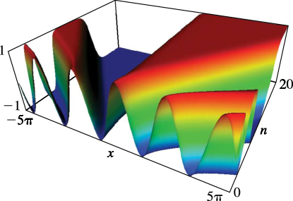
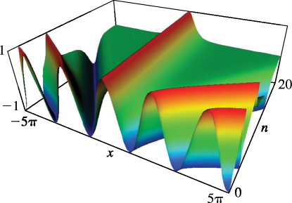
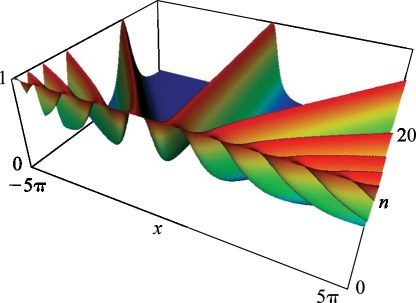
Figure 22.3.15: $\mathrm{dn}(x,k)$ for $k=1-{\mathrm{e}}^{-n}$, $n=0$ to 20, $-5\pi \le x\le 5\pi$. Magnify 3D Help

… ►

►►

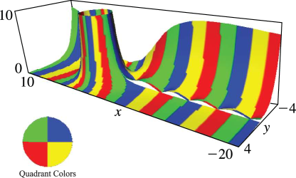
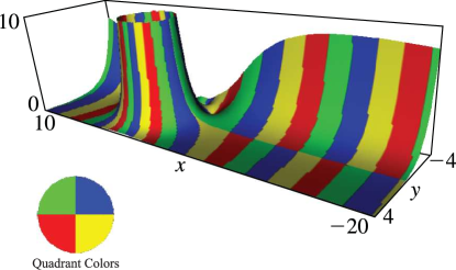
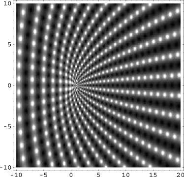
Figure 22.3.28: Density plot of $|\mathrm{sn}(20,k)|$ as a function of complex $k^2$, $-10\le \mathrm{\Re }\left(k^2\right)\le 20$, $-10\le \mathrm{\Im }\left(k^2\right)\le 10$. Grayscale, running from 0 (black) to 10 (white), with $|\mathrm{sn}(20,k)|>10$ truncated to 10. … Magnify

…

34: 26.4 Lattice Paths: Multinomial Coefficients and Set Partitions

… ►

Table 26.4.1: Multinomials and partitions.

► ►►►►

$n$	$m$	$\lambda$	$M_1$	$M_2$	$M_3$
…
$5$	$2$	$2^1,3^1$	$10$	$20$	$10$
$5$	$3$	$1^2,3^1$	$20$	$20$	$10$
…

►

…

35: 3.4 Differentiation

… ►

$$B_{-2}^5=\frac{1}{120}(6-10t-15t^2+20t^3-5t^4),$$

… ►

$$B_{-3}^6=-\frac{1}{720}(12-8t-45t^2+20t^3+15t^4-6t^5),$$

►

$$B_{-2}^6=\frac{1}{60}(9-9t-30t^2+20t^3+5t^4-3t^5),$$

… ►

$$B_2^6=-\frac{1}{60}(9+9t-30t^2-20t^3+5t^4+3t^5),$$

►

$$B_3^6=\frac{1}{720}(12+8t-45t^2-20t^3+15t^4+6t^5).$$

…

36: 6.16 Mathematical Applications

… ►

►►

Figure 6.16.2: The logarithmic integral $\mathrm{li}\left(x\right)$, together with vertical bars indicating the value of $\pi (x)$ for $x=10,20,\mathrm{\dots },1000$. Magnify

37: 26.3 Lattice Paths: Binomial Coefficients

… ►

Table 26.3.1: Binomial coefficients $\left(\genfrac{}{}{0.0pt}{}{m}{n}\right)$.

► ►►►

$m$	$n$
	…
6	1	6	15	20	15	6	1
…

►

►

Table 26.3.2: Binomial coefficients $\left(\genfrac{}{}{0.0pt}{}{m+n}{m}\right)$ for lattice paths.

► ►►►

$m$	$n$
	…
3	1	4	10	20	35	56	84	120	165
…

►

…

38: 5.22 Tables

… ►Abramowitz and Stegun (1964, Chapter 6) tabulates $\mathrm{\Gamma }\left(x\right)$, $\ln \mathrm{\Gamma }\left(x\right)$, $\psi \left(x\right)$, and ${\psi }^{\prime }\left(x\right)$ for $x=1(.005)2$ to 10D; ${\psi }^{\prime \prime }\left(x\right)$ and ${\psi }^{(3)}\left(x\right)$ for $x=1(.01)2$ to 10D; $\mathrm{\Gamma }\left(n\right)$, $1/\mathrm{\Gamma }\left(n\right)$, $\mathrm{\Gamma }\left(n+\frac{1}{2}\right)$, $\psi \left(n\right)$, ${\log }_{10}\mathrm{\Gamma }\left(n\right)$, ${\log }_{10}\mathrm{\Gamma }\left(n+\frac{1}{3}\right)$, ${\log }_{10}\mathrm{\Gamma }\left(n+\frac{1}{2}\right)$, and ${\log }_{10}\mathrm{\Gamma }\left(n+\frac{2}{3}\right)$ for $n=1(1)101$ to 8–11S; $\mathrm{\Gamma }\left(n+1\right)$ for $n=100(100)1000$ to 20S. …

39: 10.3 Graphics

… ►

►

►

Figure 10.3.14: $H_5^{(1)}\left(x+\mathrm{i}y\right)$, $-20\le x\le 10$, $-4\le y\le 4$. … Magnify 3D Help

… ►

►

►

Figure 10.3.16: $H_{5.5}^{(1)}\left(x+\mathrm{i}y\right)$, $-20\le x\le 10$, $-4\le y\le 4$. … Magnify 3D Help

…

40: 12.19 Tables

… ►

Murzewski and Sowa (1972) includes $D_{-n}\left(x\right)$ $\left(=U(n-\frac{1}{2},x)\right)$ for $n=1(1)20$, $x=0(.05)3$, 7S.

…