DLMF: Untitled Document

§17.5 ${{}_{0}\phi_{0}},{{}_{1}\phi_{0}},{{}_{1}\phi_{1}}$ Functions

… ►

17.5.1

{{}_{0}\phi_{0}}\left(-;-;q,z\right)=\sum_{n=0}^{\infty}\frac{(-1)^{n}q^{% \genfrac{(}{)}{0.0pt}{}{n}{2}}z^{n}}{\left(q;q\right)_{n}}=\left(z;q\right)_{% \infty};

ⓘ

Symbols:: $\genfrac{(}{)}{0.0pt}{}{\NVar{m}}{\NVar{n}}$ : binomial coefficient, $\left(\NVar{a};\NVar{q}\right)_{\NVar{n}}$ : $q$ -Pochhammer symbol (or $q$ -shifted factorial), ${{}_{\NVar{r+1}}\phi_{\NVar{s}}}\left(\NVar{a_{0},\dots,a_{r}};\NVar{b_{1},% \dots,b_{s}};\NVar{q},\NVar{z}\right)$ or ${{}_{\NVar{r+1}}\phi_{\NVar{s}}}\left({\NVar{a_{0},\dots,a_{r}}\atop\NVar{b_{1% },\dots,b_{s}}};\NVar{q},\NVar{z}\right)$ : basic hypergeometric (or $q$ -hypergeometric) function, $q$ : complex base, $n$ : nonnegative integer and $z$ : complex variable
Referenced by:: §17.2(iii), Erratum (V1.1.11) for Equation (17.5.1)
Permalink:: http://dlmf.nist.gov/17.5.E1
Encodings:: pMML, png, TeX
Correction (effective with 1.1.11):: The constraint $|z|<1$ is not necessary and was removed.
See also:: Annotations for §17.5, §17.5 and Ch.17

… ►

17.5.2

{{}_{1}\phi_{0}}\left(a;-;q,z\right)=\frac{\left(az;q\right)_{\infty}}{\left(z% ;q\right)_{\infty}},

|z|<1

;

ⓘ

Symbols:: $\left(\NVar{a};\NVar{q}\right)_{\NVar{n}}$ : $q$ -Pochhammer symbol (or $q$ -shifted factorial), ${{}_{\NVar{r+1}}\phi_{\NVar{s}}}\left(\NVar{a_{0},\dots,a_{r}};\NVar{b_{1},% \dots,b_{s}};\NVar{q},\NVar{z}\right)$ or ${{}_{\NVar{r+1}}\phi_{\NVar{s}}}\left({\NVar{a_{0},\dots,a_{r}}\atop\NVar{b_{1% },\dots,b_{s}}};\NVar{q},\NVar{z}\right)$ : basic hypergeometric (or $q$ -hypergeometric) function, $q$ : complex base and $z$ : complex variable
Permalink:: http://dlmf.nist.gov/17.5.E2
Encodings:: pMML, png, TeX
See also:: Annotations for §17.5, §17.5 and Ch.17

… ►

17.5.3

{{}_{1}\phi_{0}}\left(q^{-n};-;q,z\right)=\left(zq^{-n};q\right)_{n}.

ⓘ

Symbols:: $\left(\NVar{a};\NVar{q}\right)_{\NVar{n}}$ : $q$ -Pochhammer symbol (or $q$ -shifted factorial), ${{}_{\NVar{r+1}}\phi_{\NVar{s}}}\left(\NVar{a_{0},\dots,a_{r}};\NVar{b_{1},% \dots,b_{s}};\NVar{q},\NVar{z}\right)$ or ${{}_{\NVar{r+1}}\phi_{\NVar{s}}}\left({\NVar{a_{0},\dots,a_{r}}\atop\NVar{b_{1% },\dots,b_{s}}};\NVar{q},\NVar{z}\right)$ : basic hypergeometric (or $q$ -hypergeometric) function, $q$ : complex base, $n$ : nonnegative integer and $z$ : complex variable
Permalink:: http://dlmf.nist.gov/17.5.E3
Encodings:: pMML, png, TeX
See also:: Annotations for §17.5, §17.5 and Ch.17

… ►

17.5.4

{{}_{1}\phi_{0}}\left(0;-;q,z\right)=\sum_{n=0}^{\infty}\frac{z^{n}}{\left(q;q% \right)_{n}}=\frac{1}{\left(z;q\right)_{\infty}},

|z|<1

;

ⓘ

Symbols:: $\left(\NVar{a};\NVar{q}\right)_{\NVar{n}}$ : $q$ -Pochhammer symbol (or $q$ -shifted factorial), ${{}_{\NVar{r+1}}\phi_{\NVar{s}}}\left(\NVar{a_{0},\dots,a_{r}};\NVar{b_{1},% \dots,b_{s}};\NVar{q},\NVar{z}\right)$ or ${{}_{\NVar{r+1}}\phi_{\NVar{s}}}\left({\NVar{a_{0},\dots,a_{r}}\atop\NVar{b_{1% },\dots,b_{s}}};\NVar{q},\NVar{z}\right)$ : basic hypergeometric (or $q$ -hypergeometric) function, $q$ : complex base, $n$ : nonnegative integer and $z$ : complex variable
Referenced by:: §17.2(iii)
Permalink:: http://dlmf.nist.gov/17.5.E4
Encodings:: pMML, png, TeX
See also:: Annotations for §17.5, §17.5 and Ch.17

…

… ►Close to the origin

\mathbf{x}=\boldsymbol{{0}}

of parameter space, the series in §36.8 can be used. … ►Close to the bifurcation set but far from

\mathbf{x}=\boldsymbol{{0}}

, the uniform asymptotic approximations of §36.12 can be used. …

… ►The AGM,

M\left(a_{0},g_{0}\right)

, of two positive numbers

a_{0}

and

g_{0}

is defined in §19.8(i). …

Q_{n}

has the same sign as

a_{0}-g_{0}

for

n\geq 1

. …where

p_{0}>0

and …As

n\to\infty

,

p_{n}

and

\varepsilon_{n}

converge quadratically to

M\left(a_{0},g_{0}\right)

and 0, respectively, and

Q_{n}

converges to 0 faster than quadratically. … ►If

p=x

or

p=y

, then (19.22.20) reduces to

0=0

by (19.20.13), and if

z=x

or

z=y

then (19.22.19) reduces to

0=0

by (19.20.20) and (19.22.22). …

… ►

•

Abramowitz and Stegun (1964, Chapter 7) includes $\operatorname{erf}x$ , $(2/\sqrt{\pi})e^{-x^{2}}$ , $x\in[0,2]$ , 10D; $(2/\sqrt{\pi})e^{-x^{2}}$ , $x\in[2,10]$ , 8S; $xe^{x^{2}}\operatorname{erfc}x$ , $x^{-2}\in[0,0.25]$ , 7D; $2^{n}\Gamma\left(\frac{1}{2}n+1\right)\mathop{\mathrm{i}^{n}\mathrm{erfc}}% \left(x\right)$ , $n=1(1)6,10,11$ , $x\in[0,5]$ , 6S; $F\left(x\right)$ , $x\in[0,2]$ , 10D; $xF\left(x\right)$ , $x^{-2}\in[0,0.25]$ , 9D; $C\left(x\right)$ , $S\left(x\right)$ , $x\in[0,5]$ , 7D; $\mathrm{f}\left(x\right)$ , $\mathrm{g}\left(x\right)$ , $x\in[0,1]$ , $x^{-1}\in[0,1]$ , 15D.

►

•

Abramowitz and Stegun (1964, Table 27.6) includes the Goodwin–Staton integral $G\left(x\right)$ , $x=1(.1)3(.5)8$ , 4D; also $G\left(x\right)+\ln x$ , $x=0(.05)1$ , 4D.

►

•

Finn and Mugglestone (1965) includes the Voigt function $H\left(a,u\right)$ , $u\in[0,22]$ , $a\in[0,1]$ , 6S.

►

•

Zhang and Jin (1996, pp. 637, 639) includes $(2/\sqrt{\pi})e^{-x^{2}}$ , $\operatorname{erf}x$ , $x=0(.02)1(.04)3$ , 8D; $C\left(x\right)$ , $S\left(x\right)$ , $x=0(.2)10(2)100(100)500$ , 8D.

… ►

•

Abramowitz and Stegun (1964, Chapter 7) includes $w\left(z\right)$ , $x=0(.1)3.9$ , $y=0(.1)3$ , 6D.

…

… ►For

R_{F}

,

R_{G}

, and

R_{J}

, which are symmetric in

x, y, z

, we may further assume that

z

is the largest of

x, y, z

if the variables are real, then choose

z=1

, and consider only

0\leq x\leq 1

and

0\leq y\leq 1

. The cases

x=0

or

y=0

correspond to the complete integrals. … ►To view

R_{F}\left(0,y,1\right)

and

2R_{G}\left(0,y,1\right)

for complex

y

, put

y=1-k^{2}

, use (19.25.1), and see Figures 19.3.7–19.3.12. … ►To view

R_{F}\left(0,y,1\right)

and

2R_{G}\left(0,y,1\right)

for complex

y

, put

y=1-k^{2}

, use (19.25.1), and see Figures 19.3.7–19.3.12. … ►

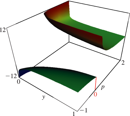
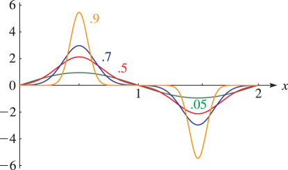
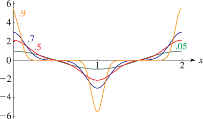
See accompanying text — Figure 19.17.8: $R_{J}\left(0,y,1,p\right)$ , $0\leq y\leq 1$ , $-1\leq p\leq 2$ . Cauchy principal values are shown when $p<0$ . … Magnify 3D Help

… ►

►

…

… ►Generalizations of the error function and Dawson’s integral are

\int_{0}^{x}e^{-t^{p}}\,\mathrm{d}t

and

\int_{0}^{x}e^{t^{p}}\,\mathrm{d}t

. …

… ►If

b

and

x

are fixed, with

b>0

and

0<x<1

, then as

a\to\infty

…for each

n=0,1,2,\dots

. … ►Then as

a\to\infty

, with

b

(

>0

) fixed, … ►with

\eta/(x-x_{0})>0

, and … ►uniformly for

b\in(0,\infty)

and

x\in(0,1)

. …

… ►If

a

,

b

,

c

are real,

a

,

b

,

c

,

c-a

,

c-b\neq 0,-1,-2,\dots

, and, without loss of generality,

b\geq a

,

c\geq a+b

(compare (15.8.1)), then ►

15.13.1

N(a,b,c)=\begin{cases}0,&a>0,\\ \left\lfloor-a\right\rfloor+\tfrac{1}{2}(1+S),&a<0,c-a>0,\\ \left\lfloor-a\right\rfloor+\tfrac{1}{2}(1+S)+\left\lfloor a-c+1\right\rfloor S% ,&a<0,c-a<0,\\ \end{cases}

ⓘ

Symbols:: $\left\lfloor\NVar{x}\right\rfloor$ : floor of $x$ , $a$ : real or complex parameter, $b$ : real or complex parameter, $c$ : real or complex parameter, $N(a,b,c)$ : number of zeros and $S$
Permalink:: http://dlmf.nist.gov/15.13.E1
Encodings:: pMML, png, TeX
See also:: Annotations for §15.13 and Ch.15

… ►If

a

,

b

,

c

,

c-a

, or

c-b\in\{0,-1,-2,\dots\}

, then

F\left(a,b;c;z\right)

is not defined, or reduces to a polynomial, or reduces to

(1-z)^{c-a-b}

times a polynomial. …

… ►To 4D the first branch points between

a_{0}\left(q\right)

and

a_{2}\left(q\right)

are at

q_{0}=\pm\mathrm{i}1.4688

with

a_{0}\left(q_{0}\right)=a_{2}\left(q_{0}\right)=2.0886

, and between

b_{2}\left(q\right)

and

b_{4}\left(q\right)

they are at

q_{1}=\pm\mathrm{i}6.9289

with

b_{2}\left(q_{1}\right)=b_{4}\left(q_{1}\right)=11.1904

. For real

q

with

|q|<|q_{0}|

,

a_{0}\left(\mathrm{i}q\right)

and

a_{2}\left(\mathrm{i}q\right)

are real-valued, whereas for real

q

with

|q|>|q_{0}|

,

a_{0}\left(\mathrm{i}q\right)

and

a_{2}\left(\mathrm{i}q\right)

are complex conjugates. … ►For a visualization of the first branch point of

a_{0}\left(\mathrm{i}\hat{q}\right)

and

a_{2}\left(\mathrm{i}\hat{q}\right)

see Figure 28.7.1. … ►All the

a_{2n}\left(q\right)

,

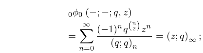
n=0,1,2,\dots

, can be regarded as belonging to a complete analytic function (in the large). …Analogous statements hold for

a_{2n+1}\left(q\right)

,

b_{2n+1}\left(q\right)

, and

b_{2n+2}\left(q\right)

, also for

n=0,1,2,\dots

. …

Lauricella%0Afunction

31—40 of 699 matching pages

31: 17.5 ${{}_{0}\phi_{0}},{{}_{1}\phi_{0}},{{}_{1}\phi_{1}}$ Functions

§17.5 ${{}_{0}\phi_{0}},{{}_{1}\phi_{0}},{{}_{1}\phi_{1}}$ Functions

32: 36.15 Methods of Computation

33: 19.22 Quadratic Transformations

34: 7.23 Tables

35: 19.17 Graphics

36: 20.3 Graphics

37: 7.16 Generalized Error Functions

38: 8.18 Asymptotic Expansions of $I_{x}\left(a,b\right)$

39: 15.13 Zeros

40: 28.7 Analytic Continuation of Eigenvalues

Lauricella%0Afunction

31—40 of 699 matching pages

31: 17.5 ϕ 0 0 , ϕ 0 1 , ϕ 1 1 Functions

§17.5 ϕ 0 0 , ϕ 0 1 , ϕ 1 1 Functions

32: 36.15 Methods of Computation

33: 19.22 Quadratic Transformations

34: 7.23 Tables

35: 19.17 Graphics

36: 20.3 Graphics

37: 7.16 Generalized Error Functions

38: 8.18 Asymptotic Expansions of I x ⁡ ( a , b )

39: 15.13 Zeros

40: 28.7 Analytic Continuation of Eigenvalues

31: 17.5 ${{}_{0}\phi_{0}},{{}_{1}\phi_{0}},{{}_{1}\phi_{1}}$ Functions

§17.5 ${{}_{0}\phi_{0}},{{}_{1}\phi_{0}},{{}_{1}\phi_{1}}$ Functions

38: 8.18 Asymptotic Expansions of $I_{x}\left(a,b\right)$