Lauricella%0Afunction
(0.002 seconds)
11—20 of 699 matching pages
11: 32.4 Isomonodromy Problems
12: 14.33 Tables
Abramowitz and Stegun (1964, Chapter 8) tabulates for , , 5–8D; for , , 5–7D; and for , , 6–8D; and for , , 6S; and for , , 6S. (Here primes denote derivatives with respect to .)
Zhang and Jin (1996, Chapter 4) tabulates for , , 7D; for , , 8D; for , , 8S; for , , 8D; for , , , , 8S; for , , 8S; for , , , 5D; for , , 7S; for , , 8S. Corresponding values of the derivative of each function are also included, as are 6D values of the first 5 -zeros of and of its derivative for , .
Belousov (1962) tabulates (normalized) for , , , 6D.
Žurina and Karmazina (1963) tabulates the conical functions for , , 7S; for , , 7S. Auxiliary tables are included to assist computation for larger values of when .
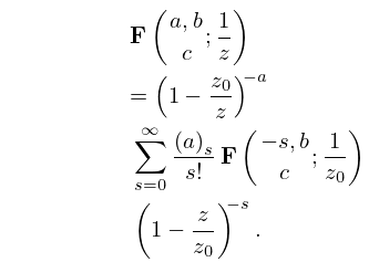
13: 15.15 Sums
14: 11.15 Approximations
Luke (1975, pp. 416–421) gives Chebyshev-series expansions for , , , and , , for ; , , , and , , ; the coefficients are to 20D.
MacLeod (1993) gives Chebyshev-series expansions for , , , and , , ; the coefficients are to 20D.
Newman (1984) gives polynomial approximations for for , , and rational-fraction approximations for for , . The maximum errors do not exceed 1.2×10⁻⁸ for the former and 2.5×10⁻⁸ for the latter.
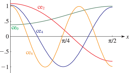
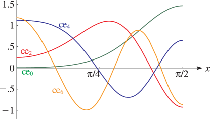
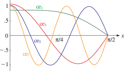
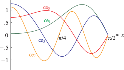
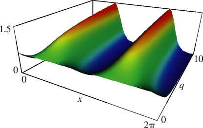
15: 28.3 Graphics
 ►
►
 ►
►
 ►
►
 ►
►
16: 32.7 Bäcklund Transformations
17: 19.37 Tables
18: 12.19 Tables
Abramowitz and Stegun (1964, Chapter 19) includes and for , , 5S; for , , 4-5D or 4-5S.
Miller (1955) includes , , and reduced derivatives for , , 8D or 8S. Modulus and phase functions, and also other auxiliary functions are tabulated.
Kireyeva and Karpov (1961) includes for , , and , , 7D.
Karpov and Čistova (1964) includes for , ; , , 6D.
Karpov and Čistova (1968) includes and for and = 0(.001 or .0001)5, , 7D or 8S.
