Lanczos tridiagonalization of a symmetric matrix

(0.003 seconds)

21—30 of 895 matching pages

21: 18.2 General Orthogonal Polynomials

… ►The matrix on the left-hand side is an (infinite tridiagonal) Jacobi matrix. This matrix is symmetric iff

c_{n}=a_{n-1}

(

n\geq 1

). … ►When the Jacobi matrix in (18.2.11_9) is truncated to an

n\times n

matrix … ►In particular, a system of OP’s on a bounded interval is always complete. …

22: 29.15 Fourier Series and Chebyshev Series

… ►A convenient way of constructing the coefficients, together with the eigenvalues, is as follows. Equations (29.6.4), with

p=1,2,\dots,n

, (29.6.3), and

A_{2n+2}=0

can be cast as an algebraic eigenvalue problem in the following way. …be the tridiagonal matrix with

\alpha_{p}

\beta_{p}

\gamma_{p}

as in (29.3.11), (29.3.12). … ►

29.15.9

[A_{1},A_{3},\dots,A_{2n+1}]^{\mathrm{T}},

ⓘ

Symbols:: $n$ : nonnegative integer and $A_{2p}$ : coefficients
Permalink:: http://dlmf.nist.gov/29.15.E9
Encodings:: pMML, png, TeX
See also:: Annotations for §29.15(i), §29.15(i), §29.15 and Ch.29

… ►The set of coefficients of this polynomial (without normalization) can also be found directly as an eigenvector of an

(n+1)\times(n+1)

tridiagonal matrix; see Arscott and Khabaza (1962). …

23: 19.31 Probability Distributions

§19.31 Probability Distributions

►

R_{G}\left(x,y,z\right)

and

R_{F}\left(x,y,z\right)

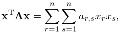
occur as the expectation values, relative to a normal probability distribution in

{\mathbb{R}}^{2}

{\mathbb{R}}^{3}

, of the square root or reciprocal square root of a quadratic form. More generally, let

\mathbf{A}

(

=[a_{r,s}]

) and

\mathbf{B}

(

=[b_{r,s}]

) be real positive-definite matrices with

n

rows and

n

columns, and let

\lambda_{1},\dots,\lambda_{n}

be the eigenvalues of

\mathbf{A}\mathbf{B}^{-1}

. If

\mathbf{x}

is a column vector with elements

x_{1},x_{2},\dots,x_{n}

and transpose

\mathbf{x}^{\mathrm{T}}

, then ►

19.31.1

\mathbf{x}^{\mathrm{T}}\mathbf{A}\mathbf{x}=\sum_{r=1}^{n}\sum_{s=1}^{n}a_{r,s% }x_{r}x_{s},

ⓘ

Symbols:: $\NVar{\mathbf{A}}^{\mathrm{T}}$ : transpose of matrix and $n$ : nonnegative integer
Permalink:: http://dlmf.nist.gov/19.31.E1
Encodings:: pMML, png, TeX
See also:: Annotations for §19.31 and Ch.19

…

24: 35.9 Applications

§35.9 Applications

… ►See James (1964), Muirhead (1982), Takemura (1984), Farrell (1985), and Chikuse (2003) for extensive treatments. … ►These references all use results related to the integral formulas (35.4.7) and (35.5.8). … ►In chemistry, Wei and Eichinger (1993) expresses the probability density functions of macromolecules in terms of generalized hypergeometric functions of matrix argument, and develop asymptotic approximations for these density functions. ►In the nascent area of applications of zonal polynomials to the limiting probability distributions of symmetric random matrices, one of the most comprehensive accounts is Rains (1998).

25: 3.8 Nonlinear Equations

… ►If

f(a)f(b)<0

with

a<b

, then the interval

[a,b]

contains one or more zeros of

f

. … ►For the computation of zeros of orthogonal polynomials as eigenvalues of finite tridiagonal matrices (§3.5(vi)), see Gil et al. (2007a, pp. 205–207). For the computation of zeros of Bessel functions, Coulomb functions, and conical functions as eigenvalues of finite parts of infinite tridiagonal matrices, see Grad and Zakrajšek (1973), Ikebe (1975), Ikebe et al. (1991), Ball (2000), and Gil et al. (2007a, pp. 205–213). … ►It is called a Julia set. In general the Julia set of an analytic function

f(z)

is a fractal, that is, a set that is self-similar. …

26: 35.10 Methods of Computation

§35.10 Methods of Computation

… ►See Yan (1992) for the

{{}_{1}F_{1}}

and

{{}_{2}F_{1}}

functions of matrix argument in the case

m=2

, and Bingham et al. (1992) for Monte Carlo simulation on

\mathbf{O}(m)

applied to a generalization of the integral (35.5.8). …

27: 1.1 Special Notation

… ► ►►►►►►

$x, y$	real variables.
…
${\mathbf{A}}^{-1}$	inverse of the square matrix $\mathbf{A}$
…
$\det(\mathbf{A})$	determinant of the square matrix $\mathbf{A}$
$\operatorname{tr}(\mathbf{A})$	trace of the square matrix $\mathbf{A}$
…
${\mathbf{A}}^{*}$	adjoint of the square matrix $\mathbf{A}$
…

►In the physics, applied maths, and engineering literature a common alternative to

\overline{a}

a^{*}

a

being a complex number or a matrix; the Hermitian conjugate of

\mathbf{A}

is usually being denoted

\mathbf{A}^{{\dagger}}

28: 1.3 Determinants, Linear Operators, and Spectral Expansions

… ►The determinant of an upper or lower triangular, or diagonal, square matrix

\mathbf{A}

is the product of the diagonal elements

\det(\mathbf{A})=\prod_{i=1}^{n}a_{ii}

. … ►The adjoint of a matrix

\mathbf{A}

is the matrix

{\mathbf{A}}^{*}

such that

\left\langle\mathbf{A}\mathbf{a},\mathbf{b}\right\rangle=\left\langle\mathbf{a% },{\mathbf{A}}^{*}\mathbf{b}\right\rangle

for all

\mathbf{a},\mathbf{b}\in\mathbf{E}_{n}

. In the case of a real matrix

{\mathbf{A}}^{*}=\mathbf{A}^{\mathrm{T}}

and in the complex case

{\mathbf{A}}^{*}={\mathbf{A}}^{{\rm H}}

. ►Real symmetric (

\mathbf{A}=\mathbf{A}^{\mathrm{T}}

) and Hermitian (

\mathbf{A}={\mathbf{A}}^{{\rm H}}

) matrices are self-adjoint operators on

\mathbf{E}_{n}

. … ►Let the columns of matrix

\mathbf{S}

be these eigenvectors

\mathbf{a}_{1},\dots,\mathbf{a}_{n}

, then

{\mathbf{S}}^{-1}={\mathbf{S}}^{{\rm H}}

, and the similarity transformation (1.2.73) is now of the form

{\mathbf{S}}^{{\rm H}}\mathbf{A}\mathbf{S}=\lambda_{i}\delta_{i,j}

. …

29: 15.17 Mathematical Applications

… ►For harmonic analysis it is more natural to represent hypergeometric functions as a Jacobi function (§15.9(ii)). …First, as spherical functions on noncompact Riemannian symmetric spaces of rank one, but also as associated spherical functions, intertwining functions, matrix elements of SL

(2,\mathbb{R})

, and spherical functions on certain nonsymmetric Gelfand pairs. Harmonic analysis can be developed for the Jacobi transform either as a generalization of the Fourier-cosine transform (§1.14(ii)) or as a specialization of a group Fourier transform. … ►By considering, as a group, all analytic transformations of a basis of solutions under analytic continuation around all paths on the Riemann sheet, we obtain the monodromy group. …For a survey of this topic see Gray (2000).

30: 18.38 Mathematical Applications

… ►

Random Matrix Theory

… ►

Zhedanov Algebra

►A symmetric Laurent polynomial is a function of the form …and

e_{1},e_{2},e_{3},e_{4}

are the elementary symmetric polynomials in

a, b, c, d

given by

a+b+c+d

ab+ac+\cdots+cd

abc+abd+acd+bcd

a b c d

, respectively. … ►The Dunkl type operator is a

q

-difference-reflection operator acting on Laurent polynomials and its eigenfunctions, the nonsymmetric Askey–Wilson polynomials, are linear combinations of the symmetric Laurent polynomial

R_{n}(z;a,b,c,d\,|\,q)

and the ‘anti-symmetric’ Laurent polynomial

z^{-1}(1-az)(1-bz)R_{n-1}(z;qa,qb,c,d\,|\,q)

, where

R_{n}(z)

is given in (18.28.1_5). …