L%E2%80%99H%C3%B4pital%20rule

SearchAdvancedHelp

(0.002 seconds)

11—20 of 325 matching pages

11: 11.4 Basic Properties

… ►where ${\mathscr{H}}_{\nu }(z)$ denotes either ${𝐇}_{\nu }\left(z\right)$ or ${𝐋}_{\nu }\left(z\right)$. … ►

${𝐋}_0^{\prime }\left(z\right)={\displaystyle \frac{2}{\pi }}+{𝐋}_1\left(z\right),$

►

${\displaystyle \frac{d}{dz}}(z{𝐋}_1\left(z\right))=z{𝐋}_0\left(z\right).$

… ►For properties of zeros of ${𝐇}_{\nu }\left(x\right)$ see Steinig (1970). ►For asymptotic expansions of zeros of ${𝐇}_0\left(x\right)$ see MacLeod (2002a).

12: 25.15 Dirichlet $L$-functions

§25.15 Dirichlet $L$-functions

►

§25.15(i) Definitions and Basic Properties

►The notation $L(s,\chi )$ was introduced by Dirichlet (1837) for the meromorphic continuation of the function defined by the series … … ►

§25.15(ii) Zeros

…

13: 23.1 Special Notation

… ► ►►►

$𝕃$	lattice in $ℂ$.
…
$G\times H$	Cartesian product of groups $G$ and $H$, that is, the set of all pairs of elements $(g,h)$ with group operation $(g_1,h_1)+(g_2,h_2)=(g_1+g_2,h_1+h_2)$.

►The main functions treated in this chapter are the Weierstrass $\mathrm{\wp }$-function $\mathrm{\wp }\left(z\right)=\mathrm{\wp }\left(z|𝕃\right)=\mathrm{\wp }(z;g_2,g_3)$; the Weierstrass zeta function $\zeta \left(z\right)=\zeta \left(z|𝕃\right)=\zeta (z;g_2,g_3)$; the Weierstrass sigma function $\sigma \left(z\right)=\sigma \left(z|𝕃\right)=\sigma (z;g_2,g_3)$; the elliptic modular function $\lambda \left(\tau \right)$; Klein’s complete invariant $J\left(\tau \right)$; Dedekind’s eta function $\eta \left(\tau \right)$. …

14: 18.39 Applications in the Physical Sciences

… ►where ${\mathrm{L}}^2$ is the (squared) angular momentum operator (14.30.12). … ►with an infinite set of orthonormal $L^2$ eigenfunctions …$p$ here being the order of the Laguerre polynomial, $L_p^{(2l+1)}$ of Table 18.8.1, line 11, and $l$ the angular momentum quantum number, and where … ►The bound state $L^2$ eigenfunctions of the radial Coulomb Schrödinger operator are discussed in §§18.39(i) and 18.39(ii), and the $\delta$-function normalized (non-$L^2$) in Chapter 33, where the solutions appear as Whittaker functions. … ►The fact that non-$L^2$ continuum scattering eigenstates may be expressed in terms or (infinite) sums of $L^2$ functions allows a reformulation of scattering theory in atomic physics wherein no non-$L^2$ functions need appear. …

15: 18.14 Inequalities

… ►

18.14.8 $${\mathrm{e}}^{-\frac{1}{2}x}\left|L_n^{(\alpha )}\left(x\right)\right|\le L_n^{(\alpha )}\left(0\right)=\frac{{\left(\alpha +1\right)}_n}{n!},$$ , $\alpha \ge 0$.

ⓘ

Symbols:

$L_n^{(\alpha )}\left(x\right)$: Laguerre (or generalized Laguerre) polynomial, ${\left(a\right)}_n$: Pochhammer’s symbol (or shifted factorial), $\mathrm{e}$: base of natural logarithm, $!$: factorial (as in $n!$), $n$: nonnegative integer and $x$: real variable

Proved:

Koornwinder (1977, Remark 4.1)(proved)

Proof sketch:

The case $\alpha =0$ follows from the result on monotonic weight functions in §18.2(xii).

A&S Ref:

22.14.13

Referenced by:

§18.14(i), §18.2(xii)

Permalink:

http://dlmf.nist.gov/18.14.E8

Encodings:

pMML, png, TeX

See also:

Annotations for §18.14(i), §18.14(i), §18.14 and Ch.18

… ►

18.14.12 $${(L_n^{(\alpha )}\left(x\right))}^2\ge L_{n-1}^{(\alpha )}\left(x\right)L_{n+1}^{(\alpha )}\left(x\right),$$ , $\alpha \ge 0$.

ⓘ

Symbols:

$L_n^{(\alpha )}\left(x\right)$: Laguerre (or generalized Laguerre) polynomial, $n$: nonnegative integer and $x$: real variable

Referenced by:

§18.14(ii)

Permalink:

http://dlmf.nist.gov/18.14.E12

Encodings:

pMML, png, TeX

See also:

Annotations for §18.14(ii), §18.14(ii), §18.14 and Ch.18

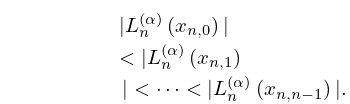
… ►Let the maxima $x_{n,m}$, $m=0,1,\mathrm{\dots },n-1$, of $|L_n^{(\alpha )}\left(x\right)|$ in $[0,\mathrm{\infty })$ be arranged so that … ►

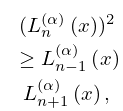
18.14.24

ⓘ

Symbols:

$L_n^{(\alpha )}\left(x\right)$: Laguerre (or generalized Laguerre) polynomial, $n$: nonnegative integer and $x$: real variable

Referenced by:

§18.14(iii)

Permalink:

http://dlmf.nist.gov/18.14.E24

Encodings:

pMML, png, TeX

See also:

Annotations for §18.14(iii), §18.14(iii), §18.14 and Ch.18

… ►The successive maxima of $|H_n\left(x\right)|$ form a decreasing sequence for $x\le 0$, and an increasing sequence for $x\ge 0$. …

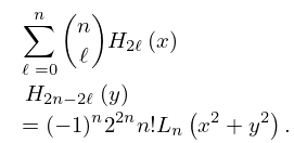
16: 18.18 Sums

… ►

Expansion of $L^2$ functions

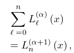
►In all three cases of Jacobi, Laguerre and Hermite, if $f(x)$ is $L^2$ on the corresponding interval with respect to the corresponding weight function and if $a_n,b_n,d_n$ are given by (18.18.1), (18.18.5), (18.18.7), respectively, then the respective series expansions (18.18.2), (18.18.4), (18.18.6) are valid with the sums converging in $L^2$ sense. … ►

18.18.12 $$\frac{L_n^{(\alpha )}\left(\lambda x\right)}{L_n^{(\alpha )}\left(0\right)}=\sum _{\mathrm{\ell }=0}^n\left(\genfrac{}{}{0.0pt}{}{n}{\mathrm{\ell }}\right){\lambda }^{\mathrm{\ell }}{(1-\lambda )}^{n-\mathrm{\ell }}\frac{L_{\mathrm{\ell }}^{(\alpha )}\left(x\right)}{L_{\mathrm{\ell }}^{(\alpha )}\left(0\right)}.$$

ⓘ

Symbols:

$L_n^{(\alpha )}\left(x\right)$: Laguerre (or generalized Laguerre) polynomial, $\left(\genfrac{}{}{0.0pt}{}{m}{n}\right)$: binomial coefficient, $\mathrm{\ell }$: nonnegative integer, $n$: nonnegative integer and $x$: real variable

Referenced by:

(18.17.34_5), §18.18(iii), §18.18(iv)

Permalink:

http://dlmf.nist.gov/18.18.E12

Encodings:

pMML, png, TeX

See also:

Annotations for §18.18(iii), §18.18(iii), §18.18 and Ch.18

… ►

18.18.37 $$\sum _{\mathrm{\ell }=0}^n{L}_{\mathrm{\ell }}^{(\alpha )}\left(x\right)=L_n^{(\alpha +1)}\left(x\right),$$

ⓘ

Symbols:

$L_n^{(\alpha )}\left(x\right)$: Laguerre (or generalized Laguerre) polynomial, $\mathrm{\ell }$: nonnegative integer, $n$: nonnegative integer and $x$: real variable

Referenced by:

§18.18(viii)

Permalink:

http://dlmf.nist.gov/18.18.E37

Encodings:

pMML, png, TeX

See also:

Annotations for §18.18(viii), §18.18(viii), §18.18 and Ch.18

… ►

18.18.40 $$\sum _{\mathrm{\ell }=0}^n\left(\genfrac{}{}{0.0pt}{}{n}{\mathrm{\ell }}\right)H_{2\mathrm{\ell }}\left(x\right)H_{2n-2\mathrm{\ell }}\left(y\right)={(-1)}^n{2}^{2n}n!L_n\left(x^2+y^2\right).$$

ⓘ

Symbols:

$H_n\left(x\right)$: Hermite polynomial, $\left(\genfrac{}{}{0.0pt}{}{m}{n}\right)$: binomial coefficient, $!$: factorial (as in $n!$), $L_n\left(x\right)=L_n^{(0)}\left(x\right)$: Laguerre polynomial, $y$: real variable, $\mathrm{\ell }$: nonnegative integer, $n$: nonnegative integer and $x$: real variable

Referenced by:

§18.18(viii)

Permalink:

http://dlmf.nist.gov/18.18.E40

Encodings:

pMML, png, TeX

See also:

Annotations for §18.18(viii), §18.18(viii), §18.18 and Ch.18

…

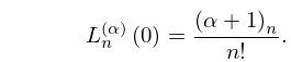
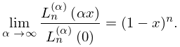
17: 18.6 Symmetry, Special Values, and Limits to Monomials

… ►

18.6.1 $$L_n^{(\alpha )}\left(0\right)=\frac{{\left(\alpha +1\right)}_n}{n!}.$$

ⓘ

Symbols:

$L_n^{(\alpha )}\left(x\right)$: Laguerre (or generalized Laguerre) polynomial, ${\left(a\right)}_n$: Pochhammer’s symbol (or shifted factorial), $!$: factorial (as in $n!$) and $n$: nonnegative integer

A&S Ref:

22.4.7 (see column for $f_n(0)$)

Referenced by:

§18.17(i), §18.6(i), §18.6(ii)

Permalink:

http://dlmf.nist.gov/18.6.E1

Encodings:

pMML, png, TeX

See also:

Annotations for §18.6(i), §18.6(i), §18.6 and Ch.18

►

Table 18.6.1: Classical OP’s: symmetry and special values.

► ►►►

$p_n(x)$	$p_n(-x)$	$p_n(1)$	$p_{2n}(0)$	$p_{2n+1}^{\prime }(0)$
…
$H_n\left(x\right)$	${(-1)}^n{H}_n\left(x\right)$		${(-1)}^n{\left(n+1\right)}_n$	$2{(-1)}^n{\left(n+1\right)}_{n+1}$
…

►

… ►

18.6.5 $$\underset{\alpha \to \mathrm{\infty }}{lim}\frac{L_n^{(\alpha )}\left(\alpha x\right)}{L_n^{(\alpha )}\left(0\right)}={(1-x)}^n.$$

ⓘ

Symbols:

$L_n^{(\alpha )}\left(x\right)$: Laguerre (or generalized Laguerre) polynomial, $n$: nonnegative integer and $x$: real variable

Referenced by:

§18.6(ii)

Permalink:

http://dlmf.nist.gov/18.6.E5

Encodings:

pMML, png, TeX

See also:

Annotations for §18.6(ii), §18.6 and Ch.18

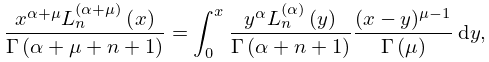
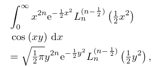
18: 18.17 Integrals

… ►

18.17.2 $${\int }_0^x{L}_m\left(y\right)L_n\left(x-y\right)dy={\int }_0^x{L}_{m+n}\left(y\right)dy=L_{m+n}\left(x\right)-L_{m+n+1}\left(x\right).$$

ⓘ

Symbols:

$dx$: differential of $x$ , $\int$: integral, $L_n\left(x\right)=L_n^{(0)}\left(x\right)$: Laguerre polynomial, $y$: real variable, $m$: nonnegative integer, $n$: nonnegative integer and $x$: real variable

Referenced by:

§18.17(i)

Permalink:

http://dlmf.nist.gov/18.17.E2

Encodings:

pMML, png, TeX

See also:

Annotations for §18.17(i), §18.17(i), §18.17 and Ch.18

… ►

18.17.14 $$\frac{x^{\alpha +\mu }{L}_n^{(\alpha +\mu )}\left(x\right)}{\mathrm{\Gamma }\left(\alpha +\mu +n+1\right)}={\int }_0^x\frac{y^{\alpha }{L}_n^{(\alpha )}\left(y\right)}{\mathrm{\Gamma }\left(\alpha +n+1\right)}\frac{{(x-y)}^{\mu -1}}{\mathrm{\Gamma }\left(\mu \right)}dy,$$ $\mu >0$, $x>0$.

ⓘ

Symbols:

$\mathrm{\Gamma }\left(z\right)$: gamma function, $L_n^{(\alpha )}\left(x\right)$: Laguerre (or generalized Laguerre) polynomial, $dx$: differential of $x$ , $\int$: integral, $y$: real variable, $n$: nonnegative integer and $x$: real variable

A&S Ref:

22.13.13

Referenced by:

§18.17(iv)

Permalink:

http://dlmf.nist.gov/18.17.E14

Encodings:

pMML, png, TeX

See also:

Annotations for §18.17(iv), §18.17(iv), §18.17 and Ch.18

►

18.17.15 $${\mathrm{e}}^{-x}{L}_n^{(\alpha )}\left(x\right)={\int }_x^{\mathrm{\infty }}{\mathrm{e}}^{-y}{L}_n^{(\alpha +\mu )}\left(y\right)\frac{{(y-x)}^{\mu -1}}{\mathrm{\Gamma }\left(\mu \right)}dy,$$ $\mu >0$.

ⓘ

Symbols:

$\mathrm{\Gamma }\left(z\right)$: gamma function, $L_n^{(\alpha )}\left(x\right)$: Laguerre (or generalized Laguerre) polynomial, $dx$: differential of $x$ , $\mathrm{e}$: base of natural logarithm, $\int$: integral, $y$: real variable, $n$: nonnegative integer and $x$: real variable

Referenced by:

§18.17(iv), §18.17(iv)

Permalink:

http://dlmf.nist.gov/18.17.E15

Encodings:

pMML, png, TeX

See also:

Annotations for §18.17(iv), §18.17(iv), §18.17 and Ch.18

… ►

18.17.30 $${\int }_0^{\mathrm{\infty }}{x}^{2n}{\mathrm{e}}^{-\frac{1}{2}{x}^2}{L}_n^{(n-\frac{1}{2})}\left(\frac{1}{2}{x}^2\right)\cos \left(xy\right)dx=\sqrt{\frac{1}{2}\pi }{y}^{2n}{\mathrm{e}}^{-\frac{1}{2}{y}^2}{L}_n^{(n-\frac{1}{2})}\left(\frac{1}{2}{y}^2\right),$$

ⓘ

Symbols:

$L_n^{(\alpha )}\left(x\right)$: Laguerre (or generalized Laguerre) polynomial, $\pi$: the ratio of the circumference of a circle to its diameter, $\cos z$: cosine function, $dx$: differential of $x$ , $\mathrm{e}$: base of natural logarithm, $\int$: integral, $y$: real variable, $n$: nonnegative integer and $x$: real variable

Referenced by:

§18.17(v)

Permalink:

http://dlmf.nist.gov/18.17.E30

Encodings:

pMML, png, TeX

See also:

Annotations for §18.17(v), §18.17(v), §18.17 and Ch.18

… ►

18.17.47 $${\int }_0^x{t}^{\alpha }\frac{L_m^{(\alpha )}\left(t\right)}{L_m^{(\alpha )}\left(0\right)}{(x-t)}^{\beta }\frac{L_n^{(\beta )}\left(x-t\right)}{L_n^{(\beta )}\left(0\right)}dt=\frac{\mathrm{\Gamma }\left(\alpha +1\right)\mathrm{\Gamma }\left(\beta +1\right)}{\mathrm{\Gamma }\left(\alpha +\beta +2\right)}{x}^{\alpha +\beta +1}\frac{L_{m+n}^{(\alpha +\beta +1)}\left(x\right)}{L_{m+n}^{(\alpha +\beta +1)}\left(0\right)}.$$

ⓘ

Symbols:

$\mathrm{\Gamma }\left(z\right)$: gamma function, $L_n^{(\alpha )}\left(x\right)$: Laguerre (or generalized Laguerre) polynomial, $dx$: differential of $x$ , $\int$: integral, $t$: real variable, $m$: nonnegative integer, $n$: nonnegative integer and $x$: real variable

Referenced by:

§18.17(viii)

Permalink:

http://dlmf.nist.gov/18.17.E47

Encodings:

pMML, png, TeX

See also:

Annotations for §18.17(viii), §18.17(viii), §18.17 and Ch.18

…

19: 18.1 Notation

… ►

Laguerre: $L_n^{(\alpha )}\left(x\right)$ and $L_n\left(x\right)=L_n^{(0)}\left(x\right)$. ($L_n^{(\alpha )}\left(x\right)$ with $\alpha \ne 0$ is also called Generalized Laguerre.)

►

Hermite: $H_n\left(x\right)$, ${\mathrm{𝐻𝑒}}_n\left(x\right)$.

… ►

$q$-Laguerre: $L_n^{(\alpha )}(x;q)$.

… ►

Continuous $q$-Hermite: $H_n\left(x|q\right)$.

…

20: 18.9 Recurrence Relations and Derivatives

… ►

18.9.13 $$L_n^{(\alpha )}\left(x\right)=L_n^{(\alpha +1)}\left(x\right)-L_{n-1}^{(\alpha +1)}\left(x\right),$$

ⓘ

Symbols:

$L_n^{(\alpha )}\left(x\right)$: Laguerre (or generalized Laguerre) polynomial, $n$: nonnegative integer and $x$: real variable

A&S Ref:

22.7.30

Referenced by:

§18.17(i), §18.9(ii), §18.9(ii)

Permalink:

http://dlmf.nist.gov/18.9.E13

Encodings:

pMML, png, TeX

See also:

Annotations for §18.9(ii), §18.9(ii), §18.9 and Ch.18

►

18.9.14 $$x{L}_n^{(\alpha +1)}\left(x\right)=-(n+1)L_{n+1}^{(\alpha )}\left(x\right)+(n+\alpha +1)L_n^{(\alpha )}\left(x\right).$$

ⓘ

Symbols:

$L_n^{(\alpha )}\left(x\right)$: Laguerre (or generalized Laguerre) polynomial, $n$: nonnegative integer and $x$: real variable

A&S Ref:

22.7.31

Referenced by:

§18.9(ii), §18.9(ii)

Permalink:

http://dlmf.nist.gov/18.9.E14

Encodings:

pMML, png, TeX

See also:

Annotations for §18.9(ii), §18.9(ii), §18.9 and Ch.18

… ►

18.9.23 $$\frac{d}{dx}{L}_n^{(\alpha )}\left(x\right)=-L_{n-1}^{(\alpha +1)}\left(x\right),$$

ⓘ

Symbols:

$L_n^{(\alpha )}\left(x\right)$: Laguerre (or generalized Laguerre) polynomial, $\frac{df}{dx}$: derivative of $f$ with respect to $x$ , $n$: nonnegative integer and $x$: real variable

Referenced by:

§18.17(i), §18.39(ii), §18.9(iii)

Permalink:

http://dlmf.nist.gov/18.9.E23

Encodings:

pMML, png, TeX

See also:

Annotations for §18.9(iii), §18.9(iii), §18.9 and Ch.18

►

18.9.24 $$\frac{d}{dx}\left({\mathrm{e}}^{-x}{x}^{\alpha }{L}_n^{(\alpha )}\left(x\right)\right)=(n+1){\mathrm{e}}^{-x}{x}^{\alpha -1}{L}_{n+1}^{(\alpha -1)}\left(x\right).$$

ⓘ

Symbols:

$L_n^{(\alpha )}\left(x\right)$: Laguerre (or generalized Laguerre) polynomial, $\frac{df}{dx}$: derivative of $f$ with respect to $x$ , $\mathrm{e}$: base of natural logarithm, $n$: nonnegative integer and $x$: real variable

Referenced by:

§18.9(iii)

Permalink:

http://dlmf.nist.gov/18.9.E24

Encodings:

pMML, png, TeX

See also:

Annotations for §18.9(iii), §18.9(iii), §18.9 and Ch.18

… ►

18.9.25 $$\frac{d}{dx}{H}_n\left(x\right)=2n{H}_{n-1}\left(x\right),$$

ⓘ

Symbols:

$H_n\left(x\right)$: Hermite polynomial, $\frac{df}{dx}$: derivative of $f$ with respect to $x$ , $n$: nonnegative integer and $x$: real variable

A&S Ref:

22.8.7

Referenced by:

§18.17(i), §18.9(iii)

Permalink:

http://dlmf.nist.gov/18.9.E25

Encodings:

pMML, png, TeX

See also:

Annotations for §18.9(iii), §18.9(iii), §18.9 and Ch.18

…