Helmholtz%20equation

SearchAdvancedHelp

(0.001 seconds)

11—20 of 499 matching pages

11: 12.17 Physical Applications

§12.17 Physical Applications

►The main applications of PCFs in mathematical physics arise when solving the Helmholtz equation …The first two equations can be transformed into (12.2.2) or (12.2.3). ►In a similar manner coordinates of the paraboloid of revolution transform the Helmholtz equation into equations related to the differential equations considered in this chapter. …

12: 28.32 Mathematical Applications

… ►The two-dimensional wave equation … ► … ►

§28.32(ii) Paraboloidal Coordinates

… ►When the Helmholtz equation …

13: 28 Mathieu Functions and Hill’s Equation

Chapter 28 Mathieu Functions and Hill’s Equation

…

14: 20 Theta Functions

Chapter 20 Theta Functions

…

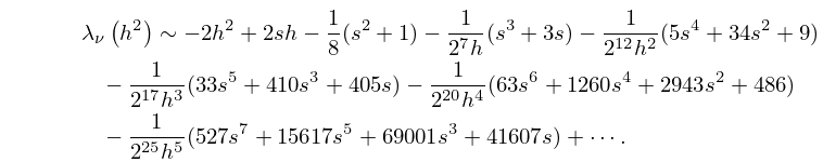
15: 28.16 Asymptotic Expansions for Large $q$

§28.16 Asymptotic Expansions for Large $q$

… ►

28.16.1 $${\lambda }_{\nu }\left(h^2\right)\sim -2h^2+2sh-\frac{1}{8}(s^2+1)-\frac{1}{2^{7}h}(s^3+3s)-\frac{1}{2^{12}{h}^2}(5s^4+34s^2+9)-\frac{1}{2^{17}{h}^3}(33s^5+410s^3+405s)-\frac{1}{2^{20}{h}^4}(63s^6+1260s^4+2943s^2+486)-\frac{1}{2^{25}{h}^5}(527s^7+15617s^5+69001s^3+41607s)+\mathrm{\cdots }.$$

ⓘ

Symbols:

${\lambda }_{\nu +2n}\left(q\right)$: eigenvalues of Mathieu equation, $\sim$: Poincaré asymptotic expansion, $h$: parameter and $\nu$: complex parameter

Permalink:

http://dlmf.nist.gov/28.16.E1

Encodings:

pMML, png, TeX

See also:

Annotations for §28.16 and Ch.28

…

16: Bibliography O

… ►

Studies on the Painlevé equations. I. Sixth Painlevé equation $P_{\mathrm{VI}}$ . Ann. Mat. Pura Appl. (4) 146, pp. 337–381.

ⓘ

External Links:

ISSN 0003-4622, Document, MathReview (Hélène Airault), ZentralBlatt

Referenced by:

§32.10(vi), §32.6(v), §32.7(vii), §32.7(viii).

Encodings:

BibTeX

►

Studies on the Painlevé equations. II. Fifth Painlevé equation $P_{\mathrm{V}}$ . Japan. J. Math. (N.S.) 13 (1), pp. 47–76.

ⓘ

External Links:

ISSN 0289-2316, MathReview (Hélène Airault), ZentralBlatt

Referenced by:

§32.10(v), §32.6(v), §32.7(viii).

Encodings:

BibTeX

►

Studies on the Painlevé equations. IV. Third Painlevé equation $P_{\mathrm{III}}$ . Funkcial. Ekvac. 30 (2-3), pp. 305–332.

ⓘ

External Links:

ISSN 0532-8721, FullText, MathReview (Hélène Airault), ZentralBlatt

Referenced by:

§32.10(iii), §32.2(iii), §32.6(iv), §32.7(viii).

Encodings:

BibTeX

… ►

Hyperasymptotics for nonlinear ODEs. II. The first Painlevé equation and a second-order Riccati equation. Proc. R. Soc. Lond. Ser. A Math. Phys. Eng. Sci. 461 (2062), pp. 3005–3021.

ⓘ

External Links:

ISSN 1364-5021, Document, MathReview, ZentralBlatt

Referenced by:

§2.11(v), §32.12(i).

Encodings:

BibTeX

… ►

An error analysis of the modified Clenshaw method for evaluating Chebyshev and Fourier series. J. Inst. Math. Appl. 20 (3), pp. 379–391.

ⓘ

External Links:

Document, MathReview (David L. Elliott), ZentralBlatt

Referenced by:

§3.11(ii).

Encodings:

BibTeX

…

17: Bibliography N

… ►

Toda equation and its solutions in special functions. J. Phys. Soc. Japan 65 (6), pp. 1589–1597.

ⓘ

External Links:

ISSN 0031-9015, Document, MathReview, ZentralBlatt

Referenced by:

§18.38(ii).

Encodings:

BibTeX

… ►

On an integral transform involving a class of Mathieu functions. SIAM J. Math. Anal. 20 (6), pp. 1500–1513.

ⓘ

External Links:

ISSN 0036-1410, Document, MathReview (K. C. Gupta), ZentralBlatt

Referenced by:

§28.26(ii).

Encodings:

BibTeX

… ►

Reduction and evaluation of elliptic integrals. Math. Comp. 20 (94), pp. 223–231.

ⓘ

External Links:

FullText, MathReview (I. A. Stegun), ZentralBlatt

Referenced by:

§19.37(iv).

Encodings:

BibTeX

… ►

Solving equations exactly. J. Res. Nat. Bur. Standards Sect. B 71B, pp. 171–179.

ⓘ

External Links:

MathReview, ZentralBlatt

Referenced by:

§27.15.

Encodings:

BibTeX

… ►

A table of integrals of the error functions. J. Res. Nat. Bur. Standards Sect B. 73B, pp. 1–20.

ⓘ

Notes:

See for additions and corrections same journal, Sect. B 75, 149–163 (1975)

External Links:

MathReview, ZentralBlatt

Referenced by:

§7.14(iii), §7.21, §7.7(iii).

Encodings:

BibTeX

…

18: 3.8 Nonlinear Equations

… ►The equation to be solved is … ►Sometimes the equation takes the form … … ►Consider $x=20$ and $j=19$. We have $p^{\prime }(20)=19!$ and $a_{19}=1+2+\mathrm{\cdots }+20=210$. …

19: 28.18 Integrals and Integral Equations

§28.18 Integrals and Integral Equations

…

20: 28.35 Tables

§28.35 Tables

… ►

Ince (1932) includes eigenvalues $a_n$, $b_n$, and Fourier coefficients for $n=0$ or $1(1)6$, $q=0(1)10(2)20(4)40$; 7D. Also ${\mathrm{ce}}_n(x,q)$, ${\mathrm{se}}_n(x,q)$ for $q=0(1)10$, $x=1(1)90$, corresponding to the eigenvalues in the tables; 5D. Notation: $a_n={\mathrm{𝑏𝑒}}_n-2q$, $b_n={\mathrm{𝑏𝑜}}_n-2q$.

►

Kirkpatrick (1960) contains tables of the modified functions ${\mathrm{Ce}}_n(x,q)$, ${\mathrm{Se}}_{n+1}(x,q)$ for $n=0(1)5$, $q=1(1)20$, $x=0.1(.1)1$; 4D or 5D.

►

National Bureau of Standards (1967) includes the eigenvalues $a_n\left(q\right)$, $b_n\left(q\right)$ for $n=0(1)3$ with $q=0(.2)20(.5)37(1)100$, and $n=4(1)15$ with $q=0(2)100$; Fourier coefficients for ${\mathrm{ce}}_n(x,q)$ and ${\mathrm{se}}_n(x,q)$ for $n=0(1)15$, $n=1(1)15$, respectively, and various values of $q$ in the interval $[0,100]$; joining factors $g_{e,n}(\sqrt{q})$, $f_{e,n}(\sqrt{q})$ for $n=0(1)15$ with $q=0(.5\text{ to }10)100$ (but in a different notation). Also, eigenvalues for large values of $q$. Precision is generally 8D.

… ►

Zhang and Jin (1996, pp. 521–532) includes the eigenvalues $a_n\left(q\right)$, $b_{n+1}\left(q\right)$ for $n=0(1)4$, $q=0(1)50$; $n=0(1)20$ ($a$’s) or 19 ($b$’s), $q=1,3,5,10,15,25,50(50)200$. Fourier coefficients for ${\mathrm{ce}}_n(x,10)$, ${\mathrm{se}}_{n+1}(x,10)$, $n=0(1)7$. Mathieu functions ${\mathrm{ce}}_n(x,10)$, ${\mathrm{se}}_{n+1}(x,10)$, and their first $x$-derivatives for $n=0(1)4$, $x=0(5^{\circ }){90}^{\circ }$. Modified Mathieu functions ${\mathrm{Mc}}_n^{(j)}(x,\sqrt{10})$, ${\mathrm{Ms}}_{n+1}^{(j)}(x,\sqrt{10})$, and their first $x$-derivatives for $n=0(1)4$, $j=1,2$, $x=0(.2)4$. Precision is mostly 9S.

…