Hankel%20inversion%20theorem

SearchAdvancedHelp

(0.002 seconds)

11—20 of 355 matching pages

11: Bibliography

… ►

Exact linearization of a Painlevé transcendent. Phys. Rev. Lett. 38 (20), pp. 1103–1106.

ⓘ

External Links:

Document, MathReview (Mark Adler)

Referenced by:

§32.11(ii), §32.13(i), §32.13(ii), §32.13(iii), §32.5.

Encodings:

BibTeX

… ►

On the degrees of irreducible factors of higher order Bernoulli polynomials. Acta Arith. 62 (4), pp. 329–342.

ⓘ

External Links:

ISSN 0065-1036, Pdf, MathReview (L. Skula), ZentralBlatt

Referenced by:

§24.12(iii).

Encodings:

BibTeX

… ►

Application of the combined nonlinear-condensation transformation to problems in statistical analysis and theoretical physics. Comput. Phys. Comm. 150 (1), pp. 1–20.

ⓘ

Notes:

Includes algorithms for Lerch’s transcendent. C and Mathematica codes by Aksenov and Jentschura are available.

External Links:

Code, Document

Referenced by:

1st item.

Encodings:

BibTeX

… ►

Repeated integrals and derivatives of $K$ Bessel functions. SIAM J. Math. Anal. 20 (1), pp. 169–175.

ⓘ

External Links:

ISSN 0036-1410, Document, MathReview (A. Haimovici), ZentralBlatt

Referenced by:

§10.43(iii).

Encodings:

BibTeX

… ►

Algorithm 588. Fast Hankel transforms using related and lagged convolutions. ACM Trans. Math. Software 8 (4), pp. 369–370.

ⓘ

Notes:

Single-precision Fortran, maximum accuracy 8S.

External Links:

ISSN 0098-3500, Document, GAMS (module 588; package TOMS)

Referenced by:

2nd item.

Encodings:

BibTeX

…

12: Bibliography K

… ►

Algorithm 737: INTLIB: A portable Fortran 77 interval standard-function library. ACM Trans. Math. Software 20 (4), pp. 447–459.

ⓘ

External Links:

ISSN 0098-3500, Document, GAMS (module 737; package TOMS), ZentralBlatt

Referenced by:

1st item.

Encodings:

BibTeX

… ►

Calculation of the complex zeros of Hankel functions and their derivatives. Zh. Vychisl. Mat. i Mat. Fiz. 25 (11), pp. 1628–1643, 1741.

ⓘ

Notes:

English translation in U.S.S.R. Computational Math. and Math. Phys. 25(6), pp. 26–36

External Links:

ISSN 0044-4669, Document, MathReview (E. Riekstiņš), ZentralBlatt

Referenced by:

§10.21(ix), §10.74(vi), 4th item, 5th item.

Encodings:

BibTeX

… ►

Methods of computing the Riemann zeta-function and some generalizations of it. USSR Comput. Math. and Math. Phys. 20 (6), pp. 212–230.

ⓘ

External Links:

Document, MathReview (Matti Jutila), ZentralBlatt

Referenced by:

§25.18(i).

Encodings:

BibTeX

… ►

Connection formulae for asymptotics of solutions of the degenerate third Painlevé equation. I. Inverse Problems 20 (4), pp. 1165–1206.

ⓘ

External Links:

ISSN 0266-5611, Document, MathReview (Shun Shimomura), ZentralBlatt

Referenced by:

§32.11(iv).

Encodings:

BibTeX

… ►

The Askey scheme as a four-manifold with corners. Ramanujan J. 20 (3), pp. 409–439.

ⓘ

External Links:

ISSN 1382-4090, Document, FullText, MathReview (José Luis López), ZentralBlatt

Referenced by:

§18.26(v), §18.26(v).

Encodings:

BibTeX

…

13: 10.17 Asymptotic Expansions for Large Argument

… ►

§10.17(i) Hankel’s Expansions

… ► … ►

§10.17(iii) Error Bounds for Real Argument and Order

… ►

§10.17(v) Exponentially-Improved Expansions

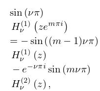
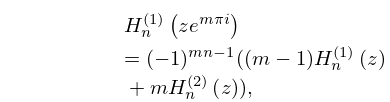
… ►For higher re-expansions of the remainder terms see Olde Daalhuis and Olver (1995a) and Olde Daalhuis (1995, 1996).

14: 10.4 Connection Formulas

§10.4 Connection Formulas

►Other solutions of (10.2.1) include $J_{-\nu }\left(z\right)$, $Y_{-\nu }\left(z\right)$, $H_{-\nu }^{(1)}\left(z\right)$, and $H_{-\nu }^{(2)}\left(z\right)$. … ►

$$H_{-n}^{(1)}\left(z\right)={(-1)}^n{H}_n^{(1)}\left(z\right),$$

►

$$H_{-n}^{(2)}\left(z\right)={(-1)}^n{H}_n^{(2)}\left(z\right).$$

… ►

$$J_{\nu }\left(z\right)=\frac{1}{2}\left(H_{\nu }^{(1)}\left(z\right)+H_{\nu }^{(2)}\left(z\right)\right),$$

…

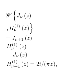
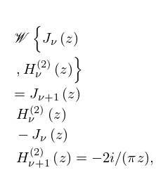
15: 10.5 Wronskians and Cross-Products

§10.5 Wronskians and Cross-Products

… ►

10.5.3 $$𝒲\left\{J_{\nu }\left(z\right),H_{\nu }^{(1)}\left(z\right)\right\}=J_{\nu +1}\left(z\right)H_{\nu }^{(1)}\left(z\right)-J_{\nu }\left(z\right)H_{\nu +1}^{(1)}\left(z\right)=2\mathrm{i}/(\pi z),$$

ⓘ

Symbols:

$J_{\nu }\left(z\right)$: Bessel function of the first kind, $H_{\nu }^{(1)}\left(z\right)$: Bessel function of the third kind (or Hankel function), $𝒲$: Wronskian, $\pi$: the ratio of the circumference of a circle to its diameter, $\mathrm{i}$: imaginary unit, $z$: complex variable and $\nu$: complex parameter

Permalink:

http://dlmf.nist.gov/10.5.E3

Encodings:

pMML, png, TeX

See also:

Annotations for §10.5 and Ch.10

►

10.5.4 $$𝒲\left\{J_{\nu }\left(z\right),H_{\nu }^{(2)}\left(z\right)\right\}=J_{\nu +1}\left(z\right)H_{\nu }^{(2)}\left(z\right)-J_{\nu }\left(z\right)H_{\nu +1}^{(2)}\left(z\right)=-2\mathrm{i}/(\pi z),$$

ⓘ

Symbols:

$J_{\nu }\left(z\right)$: Bessel function of the first kind, $H_{\nu }^{(2)}\left(z\right)$: Bessel function of the third kind (or Hankel function), $𝒲$: Wronskian, $\pi$: the ratio of the circumference of a circle to its diameter, $\mathrm{i}$: imaginary unit, $z$: complex variable and $\nu$: complex parameter

Permalink:

http://dlmf.nist.gov/10.5.E4

Encodings:

pMML, png, TeX

See also:

Annotations for §10.5 and Ch.10

►

10.5.5 $$𝒲\left\{H_{\nu }^{(1)}\left(z\right),H_{\nu }^{(2)}\left(z\right)\right\}=H_{\nu +1}^{(1)}\left(z\right)H_{\nu }^{(2)}\left(z\right)-H_{\nu }^{(1)}\left(z\right)H_{\nu +1}^{(2)}\left(z\right)=-4\mathrm{i}/(\pi z).$$

ⓘ

Symbols:

$H_{\nu }^{(1)}\left(z\right)$: Bessel function of the third kind (or Hankel function), $H_{\nu }^{(2)}\left(z\right)$: Bessel function of the third kind (or Hankel function), $𝒲$: Wronskian, $\pi$: the ratio of the circumference of a circle to its diameter, $\mathrm{i}$: imaginary unit, $z$: complex variable and $\nu$: complex parameter

A&S Ref:

9.1.17

Permalink:

http://dlmf.nist.gov/10.5.E5

Encodings:

pMML, png, TeX

See also:

Annotations for §10.5 and Ch.10

16: 10.74 Methods of Computation

… ►For evaluation of the Hankel functions $H_{\nu }^{(1)}\left(z\right)$ and $H_{\nu }^{(2)}\left(z\right)$ for complex values of $\nu$ and $z$ based on the integral representations (10.9.18) see Remenets (1973). … ► ►

§10.74(vi) Zeros and Associated Values

… ►

Hankel Transform

… ►The spherical Bessel transform is the Hankel transform (10.22.76) in the case when $\nu$ is half an odd positive integer. …

17: 27.15 Chinese Remainder Theorem

§27.15 Chinese Remainder Theorem

… ►This theorem is employed to increase efficiency in calculating with large numbers by making use of smaller numbers in most of the calculation. …Their product $m$ has 20 digits, twice the number of digits in the data. By the Chinese remainder theorem each integer in the data can be uniquely represented by its residues (mod $m_1$), (mod $m_2$), (mod $m_3$), and (mod $m_4$), respectively. …These numbers, in turn, are combined by the Chinese remainder theorem to obtain the final result $(modm)$, which is correct to 20 digits. …

18: 10.11 Analytic Continuation

§10.11 Analytic Continuation

… ►

10.11.3 $$\sin \left(\nu \pi \right)H_{\nu }^{(1)}\left(z{\mathrm{e}}^{m\pi \mathrm{i}}\right)=-\sin \left((m-1)\nu \pi \right)H_{\nu }^{(1)}\left(z\right)-{\mathrm{e}}^{-\nu \pi \mathrm{i}}\sin \left(m\nu \pi \right)H_{\nu }^{(2)}\left(z\right),$$

ⓘ

Symbols:

$H_{\nu }^{(1)}\left(z\right)$: Bessel function of the third kind (or Hankel function), $H_{\nu }^{(2)}\left(z\right)$: Bessel function of the third kind (or Hankel function), $\pi$: the ratio of the circumference of a circle to its diameter, $\mathrm{e}$: base of natural logarithm, $\mathrm{i}$: imaginary unit, $\sin z$: sine function, $m$: integer, $z$: complex variable and $\nu$: complex parameter

A&S Ref:

9.1.37

Referenced by:

§10.17(i)

Permalink:

http://dlmf.nist.gov/10.11.E3

Encodings:

pMML, png, TeX

See also:

Annotations for §10.11 and Ch.10

… ►

10.11.7 $$H_n^{(1)}\left(z{\mathrm{e}}^{m\pi \mathrm{i}}\right)={(-1)}^{mn-1}((m-1)H_n^{(1)}\left(z\right)+m{H}_n^{(2)}\left(z\right)),$$

ⓘ

Symbols:

$H_{\nu }^{(1)}\left(z\right)$: Bessel function of the third kind (or Hankel function), $H_{\nu }^{(2)}\left(z\right)$: Bessel function of the third kind (or Hankel function), $\pi$: the ratio of the circumference of a circle to its diameter, $\mathrm{e}$: base of natural logarithm, $\mathrm{i}$: imaginary unit, $m$: integer, $n$: integer and $z$: complex variable

Referenced by:

§10.17(i)

Permalink:

http://dlmf.nist.gov/10.11.E7

Encodings:

pMML, png, TeX

See also:

Annotations for §10.11 and Ch.10

►

10.11.8 $$H_n^{(2)}\left(z{\mathrm{e}}^{m\pi \mathrm{i}}\right)={(-1)}^{mn}(m{H}_n^{(1)}\left(z\right)+(m+1)H_n^{(2)}\left(z\right)).$$

ⓘ

Symbols:

$H_{\nu }^{(1)}\left(z\right)$: Bessel function of the third kind (or Hankel function), $H_{\nu }^{(2)}\left(z\right)$: Bessel function of the third kind (or Hankel function), $\pi$: the ratio of the circumference of a circle to its diameter, $\mathrm{e}$: base of natural logarithm, $\mathrm{i}$: imaginary unit, $m$: integer, $n$: integer and $z$: complex variable

Referenced by:

§10.11, §10.17(i)

Permalink:

http://dlmf.nist.gov/10.11.E8

Encodings:

pMML, png, TeX

See also:

Annotations for §10.11 and Ch.10

… ►

$H_{\nu }^{(1)}\left(\overline{z}\right)=\overline{H_{\nu }^{(2)}\left(z\right)},$ $H_{\nu }^{(2)}\left(\overline{z}\right)=\overline{H_{\nu }^{(1)}\left(z\right)}.$

…

19: 15.14 Integrals

… ►Inverse Laplace transforms of hypergeometric functions are given in Erdélyi et al. (1954a, §5.19), Oberhettinger and Badii (1973, §2.18), and Prudnikov et al. (1992b, §3.35). …Inverse Mellin transforms are given in Erdélyi et al. (1954a, §7.5). Hankel transforms of hypergeometric functions are given in Oberhettinger (1972, §1.17) and Erdélyi et al. (1954b, §8.17). …

20: 10.20 Uniform Asymptotic Expansions for Large Order

§10.20 Uniform Asymptotic Expansions for Large Order

… ►

10.20.6 $$\begin{array}{c}{H}_{\nu }^{(1)}\left(\nu z\right)\\ H_{\nu }^{(2)}\left(\nu z\right)\end{array}\}\sim 2{\mathrm{e}}^{\mp \pi \mathrm{i}/3}{\left(\frac{4\zeta }{1-z^2}\right)}^{\frac{1}{4}}\left(\frac{\mathrm{Ai}\left({\mathrm{e}}^{\pm 2\pi \mathrm{i}/3}{\nu }^{\frac{2}{3}}\zeta \right)}{{\nu }^{\frac{1}{3}}}\sum _{k=0}^{\mathrm{\infty }}\frac{A_k(\zeta )}{{\nu }^{2k}}+\frac{{\mathrm{e}}^{\pm 2\pi \mathrm{i}/3}{\mathrm{Ai}}^{\prime }\left({\mathrm{e}}^{\pm 2\pi \mathrm{i}/3}{\nu }^{\frac{2}{3}}\zeta \right)}{{\nu }^{\frac{5}{3}}}\sum _{k=0}^{\mathrm{\infty }}\frac{B_k(\zeta )}{{\nu }^{2k}}\right),$$

ⓘ

Symbols:

$\mathrm{Ai}\left(z\right)$: Airy function, $H_{\nu }^{(1)}\left(z\right)$: Bessel function of the third kind (or Hankel function), $H_{\nu }^{(2)}\left(z\right)$: Bessel function of the third kind (or Hankel function), $\sim$: Poincaré asymptotic expansion, $\pi$: the ratio of the circumference of a circle to its diameter, $\mathrm{e}$: base of natural logarithm, $\mathrm{i}$: imaginary unit, $k$: nonnegative integer, $z$: complex variable, $\nu$: complex parameter, $\zeta (z)$: solution, $A_k(\zeta )$: coefficients and $B_k(\zeta )$: coefficients

A&S Ref:

9.3.37

Referenced by:

§10.20(iii), §10.41(v)

Permalink:

http://dlmf.nist.gov/10.20.E6

Encodings:

pMML, png, TeX

See also:

Annotations for §10.20(i), §10.20 and Ch.10

… ►The curves $B{P}_1{E}_1$ and $B{P}_2{E}_2$ in the $z$-plane are the inverse maps of the line segments … ►

§10.20(iii) Double Asymptotic Properties

►For asymptotic properties of the expansions (10.20.4)–(10.20.6) with respect to large values of $z$ see §10.41(v).