Gauss%E2%80%93Christoffel%20quadrature
(0.002 seconds)
11—20 of 233 matching pages
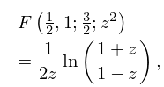
11: 15.4 Special Cases
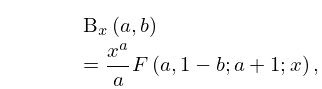
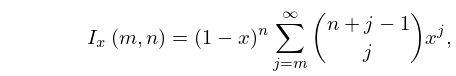
12: 8.17 Incomplete Beta Functions
…
►
8.17.7
►
8.17.8
►
8.17.9
►For the hypergeometric function see §15.2(i).
…
►
8.17.24
positive integers; .
…
13: 15.1 Special Notation
14: 15.16 Products
15: Bibliography G
…
►
Stable computation of high order Gauss quadrature rules using discretization for measures in radiation transfer.
J. Quant. Spectrosc. Radiat. Transfer 68 (2), pp. 213–223.
…
►
Algorithm 726: ORTHPOL — a package of routines for generating orthogonal polynomials and Gauss-type quadrature rules.
ACM Trans. Math. Software 20 (1), pp. 21–62.
…
►
Construction of Gauss-Christoffel quadrature formulas.
Math. Comp. 22, pp. 251–270.
…
►
Gauss quadrature approximations to hypergeometric and confluent hypergeometric functions.
J. Comput. Appl. Math. 139 (1), pp. 173–187.
…
►
Calculation of Gauss quadrature rules.
Math. Comp. 23 (106), pp. 221–230.
…
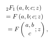
16: 15.2 Definitions and Analytical Properties
…
►
§15.2(i) Gauss Series
►The hypergeometric function is defined by the Gauss series … ►On the circle of convergence, , the Gauss series: … ►The same properties hold for , except that as a function of , in general has poles at . … ►Formula (15.4.6) reads . …17: 16.6 Transformations of Variable
…
►
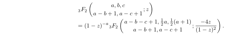
16.6.1
…
►
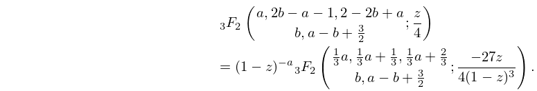
16.6.2
►For Kummer-type transformations of functions see Miller (2003) and Paris (2005a), and for further transformations see Erdélyi et al. (1953a, §4.5), Miller and Paris (2011), Choi and Rathie (2013) and Wang and Rathie (2013).
18: 16.7 Relations to Other Functions
…
►Further representations of special functions in terms of functions are given in Luke (1969a, §§6.2–6.3), and an extensive list of functions with rational numbers as parameters is given in Krupnikov and Kölbig (1997).
19: 16.10 Expansions in Series of Functions
§16.10 Expansions in Series of Functions
… ►
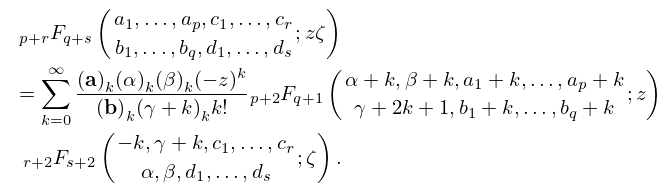
16.10.1
…
►
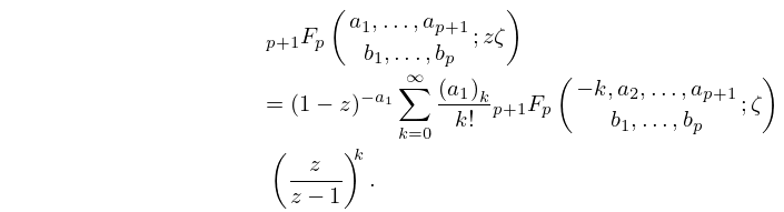
16.10.2
…
►Expansions of the form are discussed in Miller (1997), and further series of generalized hypergeometric functions are given in Luke (1969b, Chapter 9), Luke (1975, §§5.10.2 and 5.11), and Prudnikov et al. (1990, §§5.3, 6.8–6.9).
