Gaunt integral

♦ 11—20 of 422 matching pages ♦

(0.001 seconds)

11—20 of 422 matching pages

11: 10.37 Inequalities; Monotonicity

… ►See also Pal^′tsev (1999), Petropoulou (2000), Segura (2011) and Gaunt (2014).

12: Bibliography G

… ►

J. A. Gaunt (1929) The triplets of helium. Philos. Trans. Roy. Soc. London Ser. A 228, pp. 151–196.

ⓘ

External Links:: Document, ZentralBlatt (Möglich, Dr. F.)
Referenced by:: §34.3(vii).
Encodings:: BibTeX

►

R. E. Gaunt (2014) Inequalities for modified Bessel functions and their integrals. J. Math. Anal. Appl. 420 (1), pp. 373–386.

ⓘ

External Links:: ISSN 0022-247X, Document, Link, MathReview (Nihat Yagmur), ZentralBlatt
Referenced by:: §10.37, §10.37.
Encodings:: BibTeX

… ►

W. Gautschi (1973) Algorithm 471: Exponential integrals. Comm. ACM 16 (12), pp. 761–763.

ⓘ

Notes:: Includes Algol60 program, maximum accuracy 10S.
External Links:: ISSN 0001-0782, Document
Referenced by:: §6.21(ii), §8.28(vi).
Encodings:: BibTeX

… ►

M. Geller and E. W. Ng (1969) A table of integrals of the exponential integral. J. Res. Nat. Bur. Standards Sect. B 73B, pp. 191–210.

ⓘ

External Links:: MathReview (John Todd), ZentralBlatt
Referenced by:: §6.14(iii), §6.17, §6.7(iv).
Encodings:: BibTeX

… ►

M. L. Glasser (1976) Definite integrals of the complete elliptic integral

K

. J. Res. Nat. Bur. Standards Sect. B 80B (2), pp. 313–323.

ⓘ

External Links:: MathReview (H. E. Fettis), ZentralBlatt
Referenced by:: §19.13(i).
Encodings:: BibTeX

…

13: 28.18 Integrals and Integral Equations

§28.18 Integrals and Integral Equations

…

►Generalizations of elliptic integrals appear in analysis of modular theorems of Ramanujan (Anderson et al. (2000)); analysis of Selberg integrals (Van Diejen and Spiridonov (2001)); use of Legendre’s relation (19.7.1) to compute

\pi

to high precision (Borwein and Borwein (1987, p. 26)). ►

§19.35(ii) Physical

… ►

15: 6.1 Special Notation

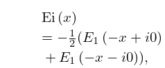
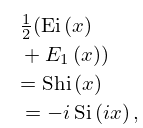
… ►Unless otherwise noted, primes indicate derivatives with respect to the argument. ►The main functions treated in this chapter are the exponential integrals

\operatorname{Ei}\left(x\right)

E_{1}\left(z\right)

, and

\operatorname{Ein}\left(z\right)

; the logarithmic integral

\operatorname{li}\left(x\right)

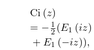
; the sine integrals

\operatorname{Si}\left(z\right)

and

\operatorname{si}\left(z\right)

; the cosine integrals

\operatorname{Ci}\left(z\right)

and

\operatorname{Cin}\left(z\right)

16: 25.7 Integrals

§25.7 Integrals

►For definite integrals of the Riemann zeta function see Prudnikov et al. (1986b, §2.4), Prudnikov et al. (1992a, §3.2), and Prudnikov et al. (1992b, §3.2).

17: 36.3 Visualizations of Canonical Integrals

§36.3 Visualizations of Canonical Integrals

►

§36.3(i) Canonical Integrals: Modulus

… ►

§36.3(ii) Canonical Integrals: Phase

►In Figure 36.3.13(a) points of confluence of phase contours are zeros of

\Psi_{2}\left(x,y\right)

; similarly for other contour plots in this subsection. In Figure 36.3.13(b) points of confluence of all colors are zeros of

\Psi_{2}\left(x,y\right)

; similarly for other density plots in this subsection. …

18: 6.14 Integrals

§6.14 Integrals

►

§6.14(i) Laplace Transforms

… ►

§6.14(ii) Other Integrals

… ►

6.14.6

\int_{0}^{\infty}{\operatorname{Ci}}^{2}\left(t\right)\,\mathrm{d}t=\int_{0}^{% \infty}{\operatorname{si}}^{2}\left(t\right)\,\mathrm{d}t=\tfrac{1}{2}\pi,

ⓘ

Symbols:: $\pi$ : the ratio of the circumference of a circle to its diameter, $\operatorname{Ci}\left(\NVar{z}\right)$ : cosine integral, $\,\mathrm{d}\NVar{x}$ : differential of $x$ , $\int$ : integral and $\operatorname{si}\left(\NVar{z}\right)$ : sine integral
A&S Ref:: 5.2.31
Permalink:: http://dlmf.nist.gov/6.14.E6
Encodings:: pMML, png, TeX
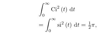
See also:: Annotations for §6.14(ii), §6.14 and Ch.6

… ►For collections of integrals, see Apelblat (1983, pp. 110–123), Bierens de Haan (1939, pp. 373–374, 409, 479, 571–572, 637, 664–673, 680–682, 685–697), Erdélyi et al. (1954a, vol. 1, pp. 40–42, 96–98, 177–178, 325), Geller and Ng (1969), Gradshteyn and Ryzhik (2000, §§5.2–5.3 and 6.2–6.27), Marichev (1983, pp. 182–184), Nielsen (1906b), Oberhettinger (1974, pp. 139–141), Oberhettinger (1990, pp. 53–55 and 158–160), Oberhettinger and Badii (1973, pp. 172–179), Prudnikov et al. (1986b, vol. 2, pp. 24–29 and 64–92), Prudnikov et al. (1992a, §§3.4–3.6), Prudnikov et al. (1992b, §§3.4–3.6), and Watrasiewicz (1967).

19: 6.17 Physical Applications

§6.17 Physical Applications

►Geller and Ng (1969) cites work with applications from diffusion theory, transport problems, the study of the radiative equilibrium of stellar atmospheres, and the evaluation of exchange integrals occurring in quantum mechanics. …Lebedev (1965) gives an application to electromagnetic theory (radiation of a linear half-wave oscillator), in which sine and cosine integrals are used.

20: 6.5 Further Interrelations

§6.5 Further Interrelations

… ►

6.5.2

\operatorname{Ei}\left(x\right)=-\tfrac{1}{2}(E_{1}\left(-x+i0\right)+E_{1}% \left(-x-i0\right)),

ⓘ

Symbols:: $E_{1}\left(\NVar{z}\right)$ : exponential integral, $\operatorname{Ei}\left(\NVar{x}\right)$ : exponential integral, $\mathrm{i}$ : imaginary unit and $x$ : real variable
A&S Ref:: 5.1.7
Referenced by:: §6.5
Permalink:: http://dlmf.nist.gov/6.5.E2
Encodings:: pMML, png, TeX
See also:: Annotations for §6.5 and Ch.6

►

6.5.3

\tfrac{1}{2}(\operatorname{Ei}\left(x\right)+E_{1}\left(x\right))=% \operatorname{Shi}\left(x\right)=-i\operatorname{Si}\left(ix\right),

ⓘ

Symbols:: $E_{1}\left(\NVar{z}\right)$ : exponential integral, $\operatorname{Ei}\left(\NVar{x}\right)$ : exponential integral, $\operatorname{Shi}\left(\NVar{z}\right)$ : hyperbolic sine integral, $\mathrm{i}$ : imaginary unit, $\operatorname{Si}\left(\NVar{z}\right)$ : sine integral and $x$ : real variable
A&S Ref:: 5.2.22 (in modified form)
Referenced by:: §6.5
Permalink:: http://dlmf.nist.gov/6.5.E3
Encodings:: pMML, png, TeX
See also:: Annotations for §6.5 and Ch.6

… ►

6.5.6

\operatorname{Ci}\left(z\right)=-\tfrac{1}{2}(E_{1}\left(iz\right)+E_{1}\left(% -iz\right)),

ⓘ

Symbols:: $\operatorname{Ci}\left(\NVar{z}\right)$ : cosine integral, $E_{1}\left(\NVar{z}\right)$ : exponential integral, $\mathrm{i}$ : imaginary unit and $z$ : complex variable
A&S Ref:: 5.2.23
Referenced by:: §6.12(ii), §6.5
Permalink:: http://dlmf.nist.gov/6.5.E6
Encodings:: pMML, png, TeX
See also:: Annotations for §6.5 and Ch.6

►

6.5.7

\mathrm{g}\left(z\right)\pm i\mathrm{f}\left(z\right)=E_{1}\left(\mp iz\right)% e^{\mp iz}.

ⓘ

Symbols:: $\mathrm{e}$ : base of natural logarithm, $E_{1}\left(\NVar{z}\right)$ : exponential integral, $\mathrm{i}$ : imaginary unit, $\mathrm{f}\left(\NVar{z}\right)$ : auxiliary function for sine and cosine integrals, $\mathrm{g}\left(\NVar{z}\right)$ : auxiliary function for sine and cosine integrals and $z$ : complex variable
Referenced by:: §6.11, §6.5, §6.7(iii)
Permalink:: http://dlmf.nist.gov/6.5.E7
Encodings:: pMML, png, TeX
See also:: Annotations for §6.5 and Ch.6