About the Project

Fourier%20cosine%20and%20sine%20transforms

AdvancedHelp

(0.004 seconds)

1—10 of 353 matching pages

1: 8.21 Generalized Sine and Cosine Integrals
§8.21 Generalized Sine and Cosine Integrals
§8.21(iv) Interrelations
§8.21(v) Special Values
§8.21(viii) Asymptotic Expansions
2: 6.2 Definitions and Interrelations
§6.2(ii) Sine and Cosine Integrals
Values at Infinity
Hyperbolic Analogs of the Sine and Cosine Integrals
§6.2(iii) Auxiliary Functions
6.2.17 f ( z ) = Ci ( z ) sin z si ( z ) cos z ,
3: 20 Theta Functions
Chapter 20 Theta Functions
4: Peter L. Walker
5: 6.19 Tables
§6.19(ii) Real Variables
  • Abramowitz and Stegun (1964, Chapter 5) includes x 1 Si ( x ) , x 2 Cin ( x ) , x 1 Ein ( x ) , x 1 Ein ( x ) , x = 0 ( .01 ) 0.5 ; Si ( x ) , Ci ( x ) , Ei ( x ) , E 1 ( x ) , x = 0.5 ( .01 ) 2 ; Si ( x ) , Ci ( x ) , x e x Ei ( x ) , x e x E 1 ( x ) , x = 2 ( .1 ) 10 ; x f ( x ) , x 2 g ( x ) , x e x Ei ( x ) , x e x E 1 ( x ) , x 1 = 0 ( .005 ) 0.1 ; Si ( π x ) , Cin ( π x ) , x = 0 ( .1 ) 10 . Accuracy varies but is within the range 8S–11S.

  • Zhang and Jin (1996, pp. 652, 689) includes Si ( x ) , Ci ( x ) , x = 0 ( .5 ) 20 ( 2 ) 30 , 8D; Ei ( x ) , E 1 ( x ) , x = [ 0 , 100 ] , 8S.

  • Abramowitz and Stegun (1964, Chapter 5) includes the real and imaginary parts of z e z E 1 ( z ) , x = 19 ( 1 ) 20 , y = 0 ( 1 ) 20 , 6D; e z E 1 ( z ) , x = 4 ( .5 ) 2 , y = 0 ( .2 ) 1 , 6D; E 1 ( z ) + ln z , x = 2 ( .5 ) 2.5 , y = 0 ( .2 ) 1 , 6D.

  • Zhang and Jin (1996, pp. 690–692) includes the real and imaginary parts of E 1 ( z ) , ± x = 0.5 , 1 , 3 , 5 , 10 , 15 , 20 , 50 , 100 , y = 0 ( .5 ) 1 ( 1 ) 5 ( 5 ) 30 , 50 , 100 , 8S.

  • 6: 6.16 Mathematical Applications
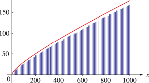
    See accompanying text
    Figure 6.16.2: The logarithmic integral li ( x ) , together with vertical bars indicating the value of π ( x ) for x = 10 , 20 , , 1000 . Magnify
    7: 6.20 Approximations
  • Hastings (1955) gives several minimax polynomial and rational approximations for E 1 ( x ) + ln x , x e x E 1 ( x ) , and the auxiliary functions f ( x ) and g ( x ) . These are included in Abramowitz and Stegun (1964, Ch. 5).

  • Cody and Thacher (1968) provides minimax rational approximations for E 1 ( x ) , with accuracies up to 20S.

  • Cody and Thacher (1969) provides minimax rational approximations for Ei ( x ) , with accuracies up to 20S.

  • MacLeod (1996b) provides rational approximations for the sine and cosine integrals and for the auxiliary functions f and g , with accuracies up to 20S.

  • Luke and Wimp (1963) covers Ei ( x ) for x 4 (20D), and Si ( x ) and Ci ( x ) for x 4 (20D).

  • 8: 8 Incomplete Gamma and Related
    Functions
    9: 28 Mathieu Functions and Hill’s Equation
    10: 8.26 Tables
  • Khamis (1965) tabulates P ( a , x ) for a = 0.05 ( .05 ) 10 ( .1 ) 20 ( .25 ) 70 , 0.0001 x 250 to 10D.

  • Abramowitz and Stegun (1964, pp. 245–248) tabulates E n ( x ) for n = 2 , 3 , 4 , 10 , 20 , x = 0 ( .01 ) 2 to 7D; also ( x + n ) e x E n ( x ) for n = 2 , 3 , 4 , 10 , 20 , x 1 = 0 ( .01 ) 0.1 ( .05 ) 0.5 to 6S.

  • Pagurova (1961) tabulates E n ( x ) for n = 0 ( 1 ) 20 , x = 0 ( .01 ) 2 ( .1 ) 10 to 4-9S; e x E n ( x ) for n = 2 ( 1 ) 10 , x = 10 ( .1 ) 20 to 7D; e x E p ( x ) for p = 0 ( .1 ) 1 , x = 0.01 ( .01 ) 7 ( .05 ) 12 ( .1 ) 20 to 7S or 7D.

  • Zhang and Jin (1996, Table 19.1) tabulates E n ( x ) for n = 1 , 2 , 3 , 5 , 10 , 15 , 20 , x = 0 ( .1 ) 1 , 1.5 , 2 , 3 , 5 , 10 , 20 , 30 , 50 , 100 to 7D or 8S.