Cauchy

SearchAdvancedHelp

(0.001 seconds)

11—20 of 36 matching pages

11: 6.2 Definitions and Interrelations

… ►

6.2.5 $$\mathrm{Ei}\left(x\right)=-{⨍}_{-x}^{\mathrm{\infty }}\frac{{\mathrm{e}}^{-t}}{t}dt={⨍}_{-\mathrm{\infty }}^x\frac{{\mathrm{e}}^t}{t}dt,$$

ⓘ

Symbols:

$dx$: differential of $x$ , $\mathrm{e}$: base of natural logarithm, $\mathrm{Ei}\left(x\right)$: exponential integral, ${⨍}_a^b$: Cauchy principal value and $x$: real variable

A&S Ref:

5.1.2

Permalink:

http://dlmf.nist.gov/6.2.E5

Encodings:

pMML, png, TeX

See also:

Annotations for §6.2(i), §6.2 and Ch.6

… ►

6.2.8 $$\mathrm{li}\left(x\right)={⨍}_0^x\frac{dt}{\ln t}=\mathrm{Ei}\left(\ln x\right),$$ $x>1$.

ⓘ

Defines:

$\mathrm{li}\left(x\right)$: logarithmic integral

Symbols:

$dx$: differential of $x$ , $\mathrm{Ei}\left(x\right)$: exponential integral, $\ln z$: principal branch of logarithm function, ${⨍}_a^b$: Cauchy principal value and $x$: real variable

A&S Ref:

5.1.3

Referenced by:

§27.12, §6.12(i)

Permalink:

http://dlmf.nist.gov/6.2.E8

Encodings:

pMML, png, TeX

See also:

Annotations for §6.2(i), §6.2 and Ch.6

…

12: 2.10 Sums and Sequences

… ►For an extension to integrals with Cauchy principal values see Elliott (1998). … ►and Cauchy’s theorem, we have … ►These problems can be brought within the scope of §2.4 by means of Cauchy’s integral formula … ►By allowing the contour in Cauchy’s formula to expand, we find that …

13: 9.10 Integrals

… ►

9.10.19 $$\mathrm{Bi}\left(x\right)=\frac{3x^{5/4}{\mathrm{e}}^{(2/3)x^{3/2}}}{2\pi }{⨍}_0^{\mathrm{\infty }}\frac{t^{-3/4}{\mathrm{e}}^{-(2/3)t^{3/2}}\mathrm{Ai}\left(t\right)}{x^{3/2}-t^{3/2}}dt,$$ $x>0$,

ⓘ

Symbols:

$\mathrm{Ai}\left(z\right)$: Airy function, $\mathrm{Bi}\left(z\right)$: Airy function, $\pi$: the ratio of the circumference of a circle to its diameter, $dx$: differential of $x$ , $\mathrm{e}$: base of natural logarithm, ${⨍}_a^b$: Cauchy principal value and $x$: real variable

Proof sketch:

To prove this equation, combine (9.2.10) with (9.10.18).

Referenced by:

§9.5(i), Erratum (V1.0.10) for Equation (9.10.19)

Permalink:

http://dlmf.nist.gov/9.10.E19

Encodings:

pMML, png, TeX

Errata (effective with 1.0.10):

The original and incorrect version,

$$\mathrm{Bi}\left(x\right)=\frac{x^{5/4}{\mathrm{e}}^{(2/3)x^{3/2}}}{2^{5/2}\pi }{⨍}_0^{\mathrm{\infty }}\frac{t^{-1/2}{\mathrm{e}}^{-(2/3)t^{3/2}}\mathrm{Ai}\left(t\right)}{x^{3/2}-t^{3/2}}dt$$

taken from Schulten et al. (1979), has been corrected.

Reported 2015-03-20 by Walter Gautschi

See also:

Annotations for §9.10(vii), §9.10 and Ch.9

►where the last integral is a Cauchy principal value (§1.4(v)). …

14: Bibliography H

… ►

Applied and Computational Complex Analysis. Vol. 3: Discrete Fourier Analysis—Cauchy Integrals—Construction of Conformal Maps—Univalent Functions. Pure and Applied Mathematics, Wiley-Interscience [John Wiley & Sons Inc.], New York.

ⓘ

Notes:

Reprinted in 1993.

External Links:

ISBN 0-471-08703-3; 0-471-58986-1, MathReview (A. E. Heins), ZentralBlatt

Referenced by:

§1.14(v), Ch.3.

Encodings:

BibTeX

…

15: 18.40 Methods of Computation

… ►

18.40.6 $$\underset{\epsilon \to 0+}{lim}{\int }_a^b\frac{w(x)dx}{x^{\prime }+\mathrm{i}\epsilon -x}dx={⨍}_a^b\frac{w(x)dx}{x^{\prime }-x}-\mathrm{i}\pi w(x^{\prime }),$$

ⓘ

Symbols:

$dx$: differential of $x$ , $\mathrm{i}$: imaginary unit, $\int$: integral, ${⨍}_a^b$: Cauchy principal value, $w(x)$: weight function and $x$: real variable

Permalink:

http://dlmf.nist.gov/18.40.E6

Encodings:

pMML, png, TeX

See also:

Annotations for §18.40(ii), §18.40(ii), §18.40 and Ch.18

…

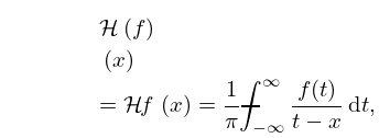
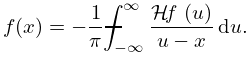
16: 1.14 Integral Transforms

… ►

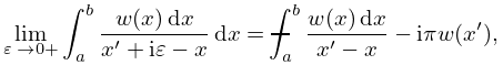
1.14.3 $$\frac{1}{2}(f(u+)+f(u-))=\frac{1}{\sqrt{2\pi }}{⨍}_{-\mathrm{\infty }}^{\mathrm{\infty }}F(x){\mathrm{e}}^{-\mathrm{i}xu}dx,$$

ⓘ

Symbols:

$\pi$: the ratio of the circumference of a circle to its diameter, $dx$: differential of $x$ , $\mathrm{e}$: base of natural logarithm, $\mathrm{i}$: imaginary unit, ${⨍}_a^b$: Cauchy principal value and $F(x)$: Fourier transform of $f(t)$

Permalink:

http://dlmf.nist.gov/1.14.E3

Encodings:

pMML, png, TeX

See also:

Annotations for §1.14(i), §1.14(i), §1.14 and Ch.1

►where the last integral denotes the Cauchy principal value (1.4.25). … ►

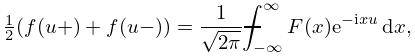
1.14.41 $$\mathscr{H}\left(f\right)\left(x\right)=\mathscr{H}f\left(x\right)=\frac{1}{\pi }{⨍}_{-\mathrm{\infty }}^{\mathrm{\infty }}\frac{f(t)}{t-x}dt,$$

ⓘ

Symbols:

$\mathscr{H}\left(f\right)\left(x\right)$: Hilbert transform, $\pi$: the ratio of the circumference of a circle to its diameter, $dx$: differential of $x$ and ${⨍}_a^b$: Cauchy principal value

Permalink:

http://dlmf.nist.gov/1.14.E41

Encodings:

pMML, png, TeX

Notational Change (effective with 1.0.15):

The notation for the Hilbert transform was changed to $\mathscr{H}\left(f\right)\left(x\right)$ or $\mathscr{H}f\left(x\right)$ from $\mathscr{H}(f;x)$.

See also:

Annotations for §1.14(v), §1.14 and Ch.1

… ►

1.14.44 $$f(x)=-\frac{1}{\pi }{⨍}_{-\mathrm{\infty }}^{\mathrm{\infty }}\frac{\mathscr{H}f\left(u\right)}{u-x}du.$$

ⓘ

Symbols:

$\mathscr{H}\left(f\right)\left(x\right)$: Hilbert transform, $\pi$: the ratio of the circumference of a circle to its diameter, $dx$: differential of $x$ and ${⨍}_a^b$: Cauchy principal value

Referenced by:

§1.14(v)

Permalink:

http://dlmf.nist.gov/1.14.E44

Encodings:

pMML, png, TeX

Notational Change (effective with 1.0.15):

The notation for the Hilbert transform was changed to $\mathscr{H}f\left(u\right)$ from $\mathscr{H}(f;u)$.

See also:

Annotations for §1.14(v), §1.14(v), §1.14 and Ch.1

… ►

Table 1.14.5: Mellin transforms.

► ►►►

$f(x)$	${\displaystyle {\int }_0^{\mathrm{\infty }}}{x}^{s-1}f(x)dx$
…
${\displaystyle \frac{1}{1-x}}$	$\pi \cot \left(s\pi \right)$,	, (Cauchy p. v.)
…

►

…

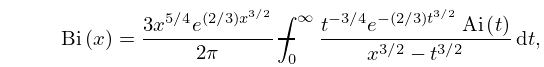
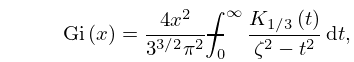
17: 9.12 Scorer Functions

… ►

9.12.23 $$\mathrm{Gi}\left(x\right)=\frac{4x^2}{3^{3/2}{\pi }^2}{⨍}_0^{\mathrm{\infty }}\frac{K_{1/3}\left(t\right)}{{\zeta }^2-t^2}dt,$$ $x>0$,

ⓘ

Symbols:

$\mathrm{Gi}\left(z\right)$: Scorer function (inhomogeneous Airy function), $\pi$: the ratio of the circumference of a circle to its diameter, $dx$: differential of $x$ , $K_{\nu }\left(z\right)$: modified Bessel function of the second kind, ${⨍}_a^b$: Cauchy principal value, $x$: real variable and $\zeta$: variable

Source:

Gordon (1970, Appendix A)

Permalink:

http://dlmf.nist.gov/9.12.E23

Encodings:

pMML, png, TeX

See also:

Annotations for §9.12(vii), §9.12 and Ch.9

►where the last integral is a Cauchy principal value (§1.4(v)). …

18: 19.20 Special Cases

… ►Cases encountered in dynamical problems are usually circular; hyperbolic cases include Cauchy principal values. If $x,y,z$ are permuted so that , then the Cauchy principal value of $R_J$ is given by …

19: Bibliography G

… ►

The solution of Cauchy’s problem for two totally hyperbolic linear differential equations by means of Riesz integrals. Ann. of Math. (2) 48 (4), pp. 785–826.

ⓘ

External Links:

FullText, MathReview (E. T. Copson), ZentralBlatt

Referenced by:

§35.2, §35.3(ii).

Encodings:

BibTeX

…

20: 4.2 Definitions

… ► …