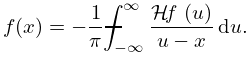
About the Project

Cauchy–Schwarz

AdvancedHelp

(0.002 seconds)

11—20 of 38 matching pages

11: 19.17 Graphics
See accompanying text
Figure 19.17.6: Cauchy principal value of R J ( x , y , 1 , 0.5 ) for 0 x 1 , y = 0 ,  0.1 ,  0.5 ,  1 . … Magnify
See accompanying text
Figure 19.17.7: Cauchy principal value of R J ( 0.5 , y , 1 , p ) for y = 0 ,  0.01 ,  0.05 ,  0.2 ,  1 , 1 p < 0 . … Magnify
See accompanying text
Figure 19.17.8: R J ( 0 , y , 1 , p ) , 0 y 1 , 1 p 2 . Cauchy principal values are shown when p < 0 . … Magnify 3D Help
12: 19.2 Definitions
The integral for E ( ϕ , k ) is well defined if k 2 = sin 2 ϕ = 1 , and the Cauchy principal value (§1.4(v)) of Π ( ϕ , α 2 , k ) is taken if 1 α 2 sin 2 ϕ vanishes at an interior point of the integration path. … If < p < 0 , then the integral in (19.2.11) is a Cauchy principal value. … where the Cauchy principal value is taken if y < 0 . Formulas involving Π ( ϕ , α 2 , k ) that are customarily different for circular cases, ordinary hyperbolic cases, and (hyperbolic) Cauchy principal values, are united in a single formula by using R C ( x , y ) . … The Cauchy principal value is hyperbolic: …
13: 19.6 Special Cases
If 1 < α 2 < , then the Cauchy principal value satisfies … Circular and hyperbolic cases, including Cauchy principal values, are unified by using R C ( x , y ) . … For the Cauchy principal value of Π ( ϕ , α 2 , k ) when α 2 > c , see §19.7(iii). …
14: 6.2 Definitions and Interrelations
6.2.5 Ei ( x ) = x e t t d t = x e t t d t ,
6.2.8 li ( x ) = 0 x d t ln t = Ei ( ln x ) , x > 1 .
15: 2.10 Sums and Sequences
For an extension to integrals with Cauchy principal values see Elliott (1998). … and Cauchy’s theorem, we have … These problems can be brought within the scope of §2.4 by means of Cauchy’s integral formula … By allowing the contour in Cauchy’s formula to expand, we find that …
16: 9.10 Integrals
9.10.19 Bi ( x ) = 3 x 5 / 4 e ( 2 / 3 ) x 3 / 2 2 π 0 t 3 / 4 e ( 2 / 3 ) t 3 / 2 Ai ( t ) x 3 / 2 t 3 / 2 d t , x > 0 ,
where the last integral is a Cauchy principal value (§1.4(v)). …
17: Bibliography H
  • P. Henrici (1986) Applied and Computational Complex Analysis. Vol. 3: Discrete Fourier Analysis—Cauchy Integrals—Construction of Conformal Maps—Univalent Functions. Pure and Applied Mathematics, Wiley-Interscience [John Wiley & Sons Inc.], New York.
  • 18: 18.40 Methods of Computation
    18.40.6 lim ε 0 + a b w ( x ) d x x + i ε x d x = a b w ( x ) d x x x i π w ( x ) ,
    19: 1.14 Integral Transforms
    1.14.3 1 2 ( f ( u + ) + f ( u ) ) = 1 2 π F ( x ) e i x u d x ,
    where the last integral denotes the Cauchy principal value (1.4.25). …
    1.14.41 ( f ) ( x ) = f ( x ) = 1 π f ( t ) t x d t ,
    1.14.44 f ( x ) = 1 π f ( u ) u x d u .
    Table 1.14.5: Mellin transforms.
    f ( x ) 0 x s 1 f ( x ) d x
    1 1 x π cot ( s π ) , 0 < s < 1 , (Cauchy p. v.)
    20: 9.12 Scorer Functions
    9.12.23 Gi ( x ) = 4 x 2 3 3 / 2 π 2 0 K 1 / 3 ( t ) ζ 2 t 2 d t , x > 0 ,
    where the last integral is a Cauchy principal value (§1.4(v)). …