.2019%E4%BD%93%E6%93%8D%E4%B8%96%E7%95%8C%E6%9D%AF%E3%80%8Ewn4.com%E3%80%8F%E4%BC%AA%E7%90%83%E8%BF%B7%E4%B8%96%E7%95%8C%E6%9D%AF%E6%AE%B5%E5%AD%90.w6n2c9o.2022%E5%B9%B411%E6%9C%8830%E6%97%A511%E6%97%B644%E5%88%8622%E7%A7%92.8ekw666qq

SearchAdvancedHelp

(0.026 seconds)

21—30 of 597 matching pages

21: 28.8 Asymptotic Expansions for Large $q$

… ►Also let $\xi =2\sqrt{h}\cos x$ and $D_m\left(\xi \right)={\mathrm{e}}^{-{\xi }^2/4}{\mathrm{𝐻𝑒}}_m\left(\xi \right)$ (§18.3). … ►

28.8.4 $$U_m(\xi )\sim D_m\left(\xi \right)-\frac{1}{2^{6}h}\left(D_{m+4}\left(\xi \right)-4!\left(\genfrac{}{}{0pt}{}{m}{4}\right)D_{m-4}\left(\xi \right)\right)+\frac{1}{2^{13}{h}^2}\left(D_{m+8}\left(\xi \right)-2^5(m+2)D_{m+4}\left(\xi \right)+4!{\mathrm{\hspace{0.17em}2}}^5(m-1)\left(\genfrac{}{}{0pt}{}{m}{4}\right)D_{m-4}\left(\xi \right)+8!\left(\genfrac{}{}{0.0pt}{}{m}{8}\right)D_{m-8}\left(\xi \right)\right)+\mathrm{\cdots },$$

ⓘ

Defines:

$U_m(\xi )$: function (locally)

Symbols:

$D_{\nu }\left(z\right)$: parabolic cylinder function, $\sim$: Poincaré asymptotic expansion, $\left(\genfrac{}{}{0.0pt}{}{m}{n}\right)$: binomial coefficient, $!$: factorial (as in $n!$), $m$: integer, $h$: parameter and $\xi$: variable

A&S Ref:

20.9.17 (in different form)

Permalink:

http://dlmf.nist.gov/28.8.E4

Encodings:

pMML, png, TeX

See also:

Annotations for §28.8(ii), §28.8 and Ch.28

►

28.8.5 $$V_m(\xi )\sim \frac{1}{2^{4}h}\left(-D_{m+2}\left(\xi \right)-m(m-1)D_{m-2}\left(\xi \right)\right)+\frac{1}{2^{10}{h}^2}\left(D_{m+6}\left(\xi \right)+(m^2-25m-36)D_{m+2}\left(\xi \right)-m(m-1)(m^2+27m-10)D_{m-2}\left(\xi \right)-6!\left(\genfrac{}{}{0.0pt}{}{m}{6}\right)D_{m-6}\left(\xi \right)\right)+\mathrm{\cdots },$$

ⓘ

Defines:

$V_m(\xi )$: function (locally)

Symbols:

$D_{\nu }\left(z\right)$: parabolic cylinder function, $\sim$: Poincaré asymptotic expansion, $\left(\genfrac{}{}{0.0pt}{}{m}{n}\right)$: binomial coefficient, $!$: factorial (as in $n!$), $m$: integer, $h$: parameter and $\xi$: variable

A&S Ref:

20.9.18 (in slightly different form)

Referenced by:

Erratum (V1.0.16) for Equation (28.8.5)

Permalink:

http://dlmf.nist.gov/28.8.E5

Encodings:

pMML, png, TeX

Error (effective with 1.0.16):

Originally the $-$ in front of the $6!$ was given incorrectly as $+$.

Suggested 2017-02-02 by Daniel Karlsson

See also:

Annotations for §28.8(ii), §28.8 and Ch.28

… ►

28.8.6 $${\widehat{C}}_m\sim {\left(\frac{\pi h}{2{(m!)}^2}\right)}^{1/4}{\left(1+\frac{2m+1}{8h}+\frac{m^4+2m^3+263m^2+262m+108}{2048h^2}+\mathrm{\cdots }\right)}^{-1/2},$$

ⓘ

Defines:

${\widehat{C}}_m$: coefficient (locally)

Symbols:

$\sim$: Poincaré asymptotic expansion, $\pi$: the ratio of the circumference of a circle to its diameter, $!$: factorial (as in $n!$), $m$: integer and $h$: parameter

A&S Ref:

20.9.19 (in slightly different form)

Permalink:

http://dlmf.nist.gov/28.8.E6

Encodings:

pMML, png, TeX

See also:

Annotations for §28.8(ii), §28.8 and Ch.28

►

28.8.7 $${\widehat{S}}_m\sim {\left(\frac{\pi h}{2{(m!)}^2}\right)}^{1/4}{\left(1-\frac{2m+1}{8h}+\frac{m^4+2m^3-121m^2-122m-84}{2048h^2}+\mathrm{\cdots }\right)}^{-1/2}.$$

ⓘ

Defines:

${\widehat{S}}_m$: coefficient (locally)

Symbols:

$\sim$: Poincaré asymptotic expansion, $\pi$: the ratio of the circumference of a circle to its diameter, $!$: factorial (as in $n!$), $m$: integer and $h$: parameter

A&S Ref:

20.9.20 (in slightly different form)

Referenced by:

§28.8(ii), Erratum (V1.1.10) for Sections 28.6(i), 28.6(ii), 28.8(i), 28.8(ii)

Permalink:

http://dlmf.nist.gov/28.8.E7

Encodings:

pMML, png, TeX

See also:

Annotations for §28.8(ii), §28.8 and Ch.28

…

22: 19.27 Asymptotic Approximations and Expansions

… ►

§19.27(ii) $R_F(x,y,z)$

… ►

§19.27(iv) $R_D(x,y,z)$

… ►

19.27.7 $$R_D(x,y,z)=\frac{3}{2z^{3/2}}\left(\ln \left(\frac{8z}{a+g}\right)-2\right)\left(1+O\left(\frac{a}{z}\right)\right),$$ $a/z\to 0$.

ⓘ

Symbols:

$O\left(x\right)$: order not exceeding, $R_D(x,y,z)$: elliptic integral symmetric in only two variables, $\ln z$: principal branch of logarithm function, $a$ and $g$

Referenced by:

§19.20(iv)

Permalink:

http://dlmf.nist.gov/19.27.E7

Encodings:

pMML, png, TeX

See also:

Annotations for §19.27(iv), §19.27 and Ch.19

►

19.27.8 $$R_D(x,y,z)=\frac{3}{\sqrt{xyz}}-\frac{6}{xy}{R}_G(x,y,0)\left(1+O\left(\frac{z}{g}\right)\right),$$ $z/g\to 0$.

ⓘ

Symbols:

$O\left(x\right)$: order not exceeding, $R_D(x,y,z)$: elliptic integral symmetric in only two variables, $R_G(x,y,z)$: symmetric elliptic integral of second kind and $g$

Referenced by:

§19.20(iv), §19.29(iii)

Permalink:

http://dlmf.nist.gov/19.27.E8

Encodings:

pMML, png, TeX

See also:

Annotations for §19.27(iv), §19.27 and Ch.19

… ►

19.27.10 $$R_D(x,y,z)=R_D(0,y,z)-\frac{3\sqrt{x}}{hz}\left(1+O\left(\sqrt{\frac{x}{h}}\right)\right),$$ $x/h\to 0$.

ⓘ

Symbols:

$O\left(x\right)$: order not exceeding, $R_D(x,y,z)$: elliptic integral symmetric in only two variables and $h$

Permalink:

http://dlmf.nist.gov/19.27.E10

Encodings:

pMML, png, TeX

See also:

Annotations for §19.27(iv), §19.27 and Ch.19

…

23: 19.29 Reduction of General Elliptic Integrals

… ►The advantages of symmetric integrals for tables of integrals and symbolic integration are illustrated by (19.29.4) and its cubic case, which replace the $8+8+12=28$ formulas in Gradshteyn and Ryzhik (2000, 3.147, 3.131, 3.152) after taking $x^2$ as the variable of integration in 3. …where the arguments of the $R_D$ function are, in order, $(a-b)(u-c)$, $(b-c)(a-u)$, $(a-b)(b-c)$. … ►The first choice gives a formula that includes the 18+9+18 = 45 formulas in Gradshteyn and Ryzhik (2000, 3.133, 3.156, 3.158), and the second choice includes the 8+8+8+12 = 36 formulas in Gradshteyn and Ryzhik (2000, 3.151, 3.149, 3.137, 3.157) (after setting $x^2=t$ in some cases). 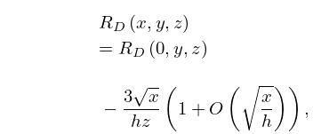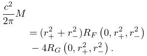… ►where …(The variables of $R_F$ are real and nonnegative unless both $Q$’s have real zeros and those of $Q_1$ interlace those of $Q_2$.) …

24: 12.3 Graphics

… ►

►►

Figure 12.3.1: $U(a,x)$, $a$ = 0. …5, 5, 8. Magnify

►

►►

Figure 12.3.2: $V(a,x)$, $a$ = 0. …5, 5, 8. Magnify

… ►

►►

Figure 12.3.5: $U(-8,x)$, $\overline{U}(-8,x)$, $F(-8,x)$, $-4\sqrt{2}\le x\le 4\sqrt{2}$. Magnify

►

►►

Figure 12.3.6: $U^{\prime }(-8,x)$, ${\overline{U}}^{\prime }(-8,x)$, $G(-8,x)$, $-4\sqrt{2}\le x\le 4\sqrt{2}$. Magnify

…

25: 17.16 Mathematical Applications

… ►More recent applications are given in Gasper and Rahman (2004, Chapter 8) and Fine (1988, Chapters 1 and 2).

26: 19.34 Mutual Inductance of Coaxial Circles

… ►

19.34.5 $$\frac{3c^2}{8\pi ab}M=3R_F(0,r_{+}^2,r_{-}^2)-2r_{-}^2{R}_D(0,r_{+}^2,r_{-}^2),$$

ⓘ

Symbols:

$R_D(x,y,z)$: elliptic integral symmetric in only two variables, $R_F(x,y,z)$: symmetric elliptic integral of first kind, $\pi$: the ratio of the circumference of a circle to its diameter, $M$: mutual inductance and $r_{\pm }$

Permalink:

http://dlmf.nist.gov/19.34.E5

Encodings:

pMML, png, TeX

See also:

Annotations for §19.34 and Ch.19

… ►

19.34.6 $$\frac{c^2}{2\pi }M=(r_{+}^2+r_{-}^2)R_F(0,r_{+}^2,r_{-}^2)-4R_G(0,r_{+}^2,r_{-}^2).$$

ⓘ

Symbols:

$R_F(x,y,z)$: symmetric elliptic integral of first kind, $R_G(x,y,z)$: symmetric elliptic integral of second kind, $\pi$: the ratio of the circumference of a circle to its diameter, $M$: mutual inductance and $r_{\pm }$

Referenced by:

§19.34

Permalink:

http://dlmf.nist.gov/19.34.E6

Encodings:

pMML, png, TeX

See also:

Annotations for §19.34 and Ch.19

… ►References for other inductance problems solvable in terms of elliptic integrals are given in Grover (1946, pp. 8 and 283).

27: 12.1 Special Notation

… ►An older notation, due to Whittaker (1902), for $U(a,z)$ is $D_{\nu }\left(z\right)$. The notations are related by $U(a,z)=D_{-a-\frac{1}{2}}\left(z\right)$. Whittaker’s notation $D_{\nu }\left(z\right)$ is useful when $\nu$ is a nonnegative integer (Hermite polynomial case).

28: 9.4 Maclaurin Series

… ►

9.4.1 $$\mathrm{Ai}\left(z\right)=\mathrm{Ai}\left(0\right)\left(1+\frac{1}{3!}{z}^3+\frac{1\cdot 4}{6!}{z}^6+\frac{1\cdot 4\cdot 7}{9!}{z}^9+\mathrm{\cdots }\right)+{\mathrm{Ai}}^{\prime }\left(0\right)\left(z+\frac{2}{4!}{z}^4+\frac{2\cdot 5}{7!}{z}^7+\frac{2\cdot 5\cdot 8}{10!}{z}^{10}+\mathrm{\cdots }\right),$$

ⓘ

Symbols:

$\mathrm{Ai}\left(z\right)$: Airy function, $!$: factorial (as in $n!$) and $z$: complex variable

Source:

Olver (1997b, p. 54)

A&S Ref:

10.4.2 (with 10.4.4 and 10.4.5)

Permalink:

http://dlmf.nist.gov/9.4.E1

Encodings:

pMML, png, TeX

See also:

Annotations for §9.4 and Ch.9

►

9.4.2 $${\mathrm{Ai}}^{\prime }\left(z\right)={\mathrm{Ai}}^{\prime }\left(0\right)\left(1+\frac{2}{3!}{z}^3+\frac{2\cdot 5}{6!}{z}^6+\frac{2\cdot 5\cdot 8}{9!}{z}^9+\mathrm{\cdots }\right)+\mathrm{Ai}\left(0\right)\left(\frac{1}{2!}{z}^2+\frac{1\cdot 4}{5!}{z}^5+\frac{1\cdot 4\cdot 7}{8!}{z}^8+\mathrm{\cdots }\right),$$

ⓘ

Symbols:

$\mathrm{Ai}\left(z\right)$: Airy function, $!$: factorial (as in $n!$) and $z$: complex variable

Proof sketch:

Use methods of Olver (1997b, p. 54).

Permalink:

http://dlmf.nist.gov/9.4.E2

Encodings:

pMML, png, TeX

See also:

Annotations for §9.4 and Ch.9

►

9.4.3 $$\mathrm{Bi}\left(z\right)=\mathrm{Bi}\left(0\right)\left(1+\frac{1}{3!}{z}^3+\frac{1\cdot 4}{6!}{z}^6+\frac{1\cdot 4\cdot 7}{9!}{z}^9+\mathrm{\cdots }\right)+{\mathrm{Bi}}^{\prime }\left(0\right)\left(z+\frac{2}{4!}{z}^4+\frac{2\cdot 5}{7!}{z}^7+\frac{2\cdot 5\cdot 8}{10!}{z}^{10}+\mathrm{\cdots }\right),$$

ⓘ

Symbols:

$\mathrm{Bi}\left(z\right)$: Airy function, $!$: factorial (as in $n!$) and $z$: complex variable

Proof sketch:

Use methods of Olver (1997b, p. 54).

A&S Ref:

10.4.3 (with 10.4.4 and 10.4.5)

Referenced by:

(9.12.15)

Permalink:

http://dlmf.nist.gov/9.4.E3

Encodings:

pMML, png, TeX

See also:

Annotations for §9.4 and Ch.9

►

9.4.4 $${\mathrm{Bi}}^{\prime }\left(z\right)={\mathrm{Bi}}^{\prime }\left(0\right)\left(1+\frac{2}{3!}{z}^3+\frac{2\cdot 5}{6!}{z}^6+\frac{2\cdot 5\cdot 8}{9!}{z}^9+\mathrm{\cdots }\right)+\mathrm{Bi}\left(0\right)\left(\frac{1}{2!}{z}^2+\frac{1\cdot 4}{5!}{z}^5+\frac{1\cdot 4\cdot 7}{8!}{z}^8+\mathrm{\cdots }\right).$$

ⓘ

Symbols:

$\mathrm{Bi}\left(z\right)$: Airy function, $!$: factorial (as in $n!$) and $z$: complex variable

Proof sketch:

Use methods of Olver (1997b, p. 54).

Permalink:

http://dlmf.nist.gov/9.4.E4

Encodings:

pMML, png, TeX

See also:

Annotations for §9.4 and Ch.9

29: 10.62 Graphs

… ►

►►

Figure 10.62.1: $\mathrm{ber}x$, $\mathrm{bei}x$, ${\mathrm{ber}}^{\prime }x$, ${\mathrm{bei}}^{\prime }x$, $0\le x\le 8$. Magnify

►

►►

Figure 10.62.2: $\ker x$, $\mathrm{kei}x$, ${\ker }^{\prime }x$, ${\mathrm{kei}}^{\prime }x$, $0\le x\le 8$. Magnify

►

►►

Figure 10.62.3: ${\mathrm{e}}^{-x/\sqrt{2}}\mathrm{ber}x$, ${\mathrm{e}}^{-x/\sqrt{2}}\mathrm{bei}x$, ${\mathrm{e}}^{-x/\sqrt{2}}M\left(x\right)$, $0\le x\le 8$. Magnify

►

►►

Figure 10.62.4: ${\mathrm{e}}^{x/\sqrt{2}}\ker x$, ${\mathrm{e}}^{x/\sqrt{2}}\mathrm{kei}x$, ${\mathrm{e}}^{x/\sqrt{2}}N\left(x\right)$, $0\le x\le 8$. Magnify

30: 19.2 Definitions

… ►

$$D(m\pi \pm \varphi ,k)=2mD\left(k\right)\pm D(\varphi ,k).$$

… ►

§19.2(iv) A Related Function: $R_C(x,y)$

… ►Formulas involving $\mathrm{\Pi }(\varphi ,{\alpha }^2,k)$ that are customarily different for circular cases, ordinary hyperbolic cases, and (hyperbolic) Cauchy principal values, are united in a single formula by using $R_C(x,y)$. … ►When $x$ and $y$ are positive, $R_C(x,y)$ is an inverse circular function if and an inverse hyperbolic function (or logarithm) if $x>y$: …For the special cases of $R_C(x,x)$ and $R_C(0,y)$ see (19.6.15). …