.%E5%9C%A8%E5%93%AA%E9%87%8C%E5%8F%AF%E4%BB%A5%E4%B9%B0%E4%B8%96%E7%95%8C%E6%9D%AF%E3%80%8Ewn4.com%E3%80%8F%E7%9C%8B%E4%B8%96%E7%95%8C%E6%9D%AF%E6%A0%87%E8%AF%AD.w6n2c9o.2022%E5%B9%B411%E6%9C%8830%E6%97%A57%E6%97%B645%E5%88%8649%E7%A7%92.gkswkagoe.gov.hk

SearchAdvancedHelp

(0.028 seconds)

21—30 of 570 matching pages

21: 18.8 Differential Equations

… ►

Table 18.8.1: Classical OP’s: differential equations $A(x)f^{\prime \prime }(x)+B(x)f^{\prime }(x)+C(x)f(x)+{\lambda }_{n}f(x)=0$.

► ►►►►►

#	$f(x)$	$A(x)$	$B(x)$	$C(x)$	${\lambda }_n$
…
4	$C_n^{(\lambda )}\left(x\right)$	$1-x^2$	$-(2\lambda +1)x$	$0$	$n(n+2\lambda )$
…
8	$L_n^{(\alpha )}\left(x\right)$	$x$	$\alpha +1-x$	$0$	$n$
9	${\mathrm{e}}^{-\frac{1}{2}{x}^2}{x}^{\alpha +\frac{1}{2}}{L}_n^{(\alpha )}\left(x^2\right)$	$1$	$0$	$-x^2+(\frac{1}{4}-{\alpha }^2)x^{-2}$	$4n+2\alpha +2$
…

►

…

22: 16.7 Relations to Other Functions

… ►For $\mathit{3}j$, $\mathit{6}j$, $\mathit{9}j$ symbols see Chapter 34. Further representations of special functions in terms of ${}_p{}^{}F_q^{}$ functions are given in Luke (1969a, §§6.2–6.3), and an extensive list of ${}_{q+1}{}^{}F_q^{}$ functions with rational numbers as parameters is given in Krupnikov and Kölbig (1997).

23: 34.8 Approximations for Large Parameters

§34.8 Approximations for Large Parameters

►For large values of the parameters in the $\mathit{3}j$, $\mathit{6}j$, and $\mathit{9}j$ symbols, different asymptotic forms are obtained depending on which parameters are large. … ►For approximations for the $\mathit{3}j$, $\mathit{6}j$, and $\mathit{9}j$ symbols with error bounds see Flude (1998), Chen et al. (1999), and Watson (1999): these references also cite earlier work.

24: 23.20 Mathematical Applications

… ►An algebraic curve that can be put either into the form … ►The addition law states that to find the sum of two points, take the third intersection with $C$ of the chord joining them (or the tangent if they coincide); then its reflection in the $x$-axis gives the required sum. … ►Then $\mathrm{\varnothing }\subseteq T\subseteq I\subseteq K\subseteq C$. Both $T,K$ are subgroups of $C$, though $I$ may not be. …The order of a point (if finite and not already determined) can have only the values 3, 5, 6, 7, 9, 10, or 12, and so can be found from $2P=-P$, $4P=-P$, $4P=-2P$, $8P=P$, $8P=-P$, $8P=-2P$, or $8P=-4P$. …

25: Bibliography T

… ►

LSFBTR: A subroutine for calculating spherical Bessel transforms. Comput. Phys. Comm. 30 (1), pp. 93–99.

ⓘ

Notes:

Single-precision Fortran.

External Links:

ISSN 0010-4655, Document, Code

Referenced by:

9th item.

Encodings:

BibTeX

… ►

The universal Askey-Wilson algebra and DAHA of type $(C_1^{\vee },C_1)$ . SIGMA 9, pp. Paper 047, 40 pp..

ⓘ

External Links:

ISSN 1815-0659, Link, MathReview (Renato Álvarez-Nodarse), ZentralBlatt

Referenced by:

§18.38(iii).

Encodings:

BibTeX

… ►

Algorithm 926: incomplete gamma functions with negative arguments. ACM Trans. Math. Software 39 (2), pp. Art. 14, 9.

ⓘ

External Links:

ISSN 0098-3500, Document, FullText, MathReview Entry, ZentralBlatt

Referenced by:

7th item, §8.28(ii).

Encodings:

BibTeX

… ►

Angular Momentum: An Illustrated Guide to Rotational Symmetries for Physical Systems. A Wiley-Interscience Publication, John Wiley & Sons Inc., New York.

ⓘ

Notes:

With 1 Macintosh floppy disk (3.5 inch; DD). Programs for the calculation of $3j,6j,9j$ symbols are included.

External Links:

ISBN 0-471-55264-X, MathReview (J. F. Cornwell), ZentralBlatt

Referenced by:

§34.3(vii).

Encodings:

BibTeX

… ►

Theory of the Fresnel integral. USSR Comput. Math. and Math. Phys. 9 (4), pp. 271–279.

ⓘ

Notes:

Translation of the paper in Zh. Vychisl. Mat. Mat. Fiz., Vol. 9, No. 4, 938-944, 1969

External Links:

Document, ZentralBlatt

Referenced by:

§7.13(iv).

Encodings:

BibTeX

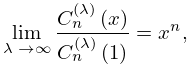
26: 18.6 Symmetry, Special Values, and Limits to Monomials

… ►

Table 18.6.1: Classical OP’s: symmetry and special values.

► ►►►

$p_n(x)$	$p_n(-x)$	$p_n(1)$	$p_{2n}(0)$	$p_{2n+1}^{\prime }(0)$
…
$C_n^{(\lambda )}\left(x\right)$	${(-1)}^n{C}_n^{(\lambda )}\left(x\right)$	${\left(2\lambda \right)}_n/n!$	${(-1)}^n{\left(\lambda \right)}_n/n!$	$2{(-1)}^n{\left(\lambda \right)}_{n+1}/n!$
…

►

… ►

18.6.4 $$\underset{\lambda \to \mathrm{\infty }}{lim}\frac{C_n^{(\lambda )}\left(x\right)}{C_n^{(\lambda )}\left(1\right)}=x^n,$$

ⓘ

Symbols:

$C_n^{(\lambda )}\left(x\right)$: ultraspherical (or Gegenbauer) polynomial, $n$: nonnegative integer and $x$: real variable

Referenced by:

§18.18(iv), §18.6(ii)

Permalink:

http://dlmf.nist.gov/18.6.E4

Encodings:

pMML, png, TeX

See also:

Annotations for §18.6(ii), §18.6 and Ch.18

…

27: 3.3 Interpolation

… ►If $f$ is analytic in a simply-connected domain $D$ (§1.13(i)), then for $z\in D$, …where $C$ is a simple closed contour in $D$ described in the positive rotational sense and enclosing the points $z,z_1,z_2,\mathrm{\dots },z_n$. … ►where ${\omega }_{n+1}(\zeta )$ is given by (3.3.3), and $C$ is a simple closed contour in $D$ described in the positive rotational sense and enclosing $z_0,z_1,\mathrm{\dots },z_n$. … ►By using this approximation to $x$ as a new point, $x_3=x$, and evaluating $\left[f_0,f_1,f_2,f_3\right]x=\mathrm{1.12388\hspace{0.33em}6190}$, we find that $x=-\mathrm{2.33810\hspace{0.33em}7409}$, with 9 correct digits. … ►Then by using $x_3$ in Newton’s interpolation formula, evaluating $\left[x_0,x_1,x_2,x_3\right]f=-\mathrm{0.26608\hspace{0.33em}28233}$ and recomputing $f^{\prime }(x)$, another application of Newton’s rule with starting value $x_3$ gives the approximation $x=\mathrm{2.33810\hspace{0.33em}7373}$, with 8 correct digits. …

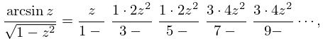
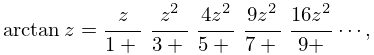
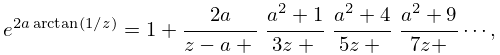
28: 4.25 Continued Fractions

… ►

4.25.2 $$\tan \left(az\right)=\frac{a\tan z}{1+}\frac{(1-a^2){\tan }^{2}z}{3+}\frac{(4-a^2){\tan }^{2}z}{5+}\frac{(9-a^2){\tan }^{2}z}{7+}\mathrm{\cdots },$$ , $az\ne \pm \frac{1}{2}\pi ,\pm \frac{3}{2}\pi ,\mathrm{\dots }$.

ⓘ

Symbols:

$\pi$: the ratio of the circumference of a circle to its diameter, $\mathrm{\Re }$: real part, $\tan z$: tangent function, $a$: real or complex constant and $z$: complex variable

A&S Ref:

4.3.95

Permalink:

http://dlmf.nist.gov/4.25.E2

Encodings:

pMML, png, TeX

See also:

Annotations for §4.25 and Ch.4

►

4.25.3 $$\frac{\arcsin z}{\sqrt{1-z^2}}=\frac{z}{1-}\frac{1\cdot 2z^2}{3-}\frac{1\cdot 2z^2}{5-}\frac{3\cdot 4z^2}{7-}\frac{3\cdot 4z^2}{9-}\mathrm{\cdots },$$

ⓘ

Symbols:

$\arcsin z$: arcsine function and $z$: complex variable

A&S Ref:

4.4.44

Permalink:

http://dlmf.nist.gov/4.25.E3

Encodings:

pMML, png, TeX

See also:

Annotations for §4.25 and Ch.4

… ►

4.25.4 $$\arctan z=\frac{z}{1+}\frac{z^2}{3+}\frac{4z^2}{5+}\frac{9z^2}{7+}\frac{16z^2}{9+}\mathrm{\cdots },$$

ⓘ

Symbols:

$\arctan z$: arctangent function and $z$: complex variable

A&S Ref:

4.4.43

Referenced by:

§3.10(ii)

Permalink:

http://dlmf.nist.gov/4.25.E4

Encodings:

pMML, png, TeX

See also:

Annotations for §4.25 and Ch.4

… ►

4.25.5 $${\mathrm{e}}^{2a\arctan \left(1/z\right)}=1+\frac{2a}{z-a+}\frac{a^2+1}{3z+}\frac{a^2+4}{5z+}\frac{a^2+9}{7z+}\mathrm{\cdots },$$

ⓘ

Symbols:

$\mathrm{e}$: base of natural logarithm, $\arctan z$: arctangent function, $a$: real or complex constant and $z$: complex variable

A&S Ref:

4.2.42

Permalink:

http://dlmf.nist.gov/4.25.E5

Encodings:

pMML, png, TeX

See also:

Annotations for §4.25 and Ch.4

…

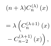
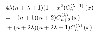
29: 18.9 Recurrence Relations and Derivatives

… ►

18.9.1 $$p_{n+1}(x)=(A_{n}x+B_n)p_n(x)-C_n{p}_{n-1}(x),$$

ⓘ

Defines:

$A_n$: coefficient (locally), $B_n$: coefficient (locally) and $C_n$: coefficient (locally)

Symbols:

$p_n(x)$: polynomial of degree $n$ , $n$: nonnegative integer and $x$: real variable

Referenced by:

§18.21(ii), Table 18.9.1, §18.9(i)

Permalink:

http://dlmf.nist.gov/18.9.E1

Encodings:

pMML, png, TeX

See also:

Annotations for §18.9(i), §18.9(i), §18.9 and Ch.18

►with initial values $p_0(x)=1$ and $p_1(x)=A_{0}x+B_0$. … ► $A_0$ and $B_0$ have to be understood for $\alpha +\beta =0$ or $-1$ by continuity in $\alpha$ and $\beta$, that is, $A_0=\frac{1}{2}(\alpha +\beta )+1$ and $B_0=\frac{1}{2}(\alpha -\beta )$. … ►

18.9.7 $$(n+\lambda )C_n^{(\lambda )}\left(x\right)=\lambda \left(C_n^{(\lambda +1)}\left(x\right)-C_{n-2}^{(\lambda +1)}\left(x\right)\right),$$

ⓘ

Symbols:

$C_n^{(\lambda )}\left(x\right)$: ultraspherical (or Gegenbauer) polynomial, $n$: nonnegative integer and $x$: real variable

Referenced by:

§18.9(ii)

Permalink:

http://dlmf.nist.gov/18.9.E7

Encodings:

pMML, png, TeX

See also:

Annotations for §18.9(ii), §18.9(ii), §18.9 and Ch.18

►

18.9.8 $$4\lambda (n+\lambda +1)(1-x^2)C_n^{(\lambda +1)}\left(x\right)=-(n+1)(n+2)C_{n+2}^{(\lambda )}\left(x\right)+(n+2\lambda )(n+2\lambda +1)C_n^{(\lambda )}\left(x\right).$$

ⓘ

Symbols:

$C_n^{(\lambda )}\left(x\right)$: ultraspherical (or Gegenbauer) polynomial, $n$: nonnegative integer and $x$: real variable

Referenced by:

§18.9(ii)

Permalink:

http://dlmf.nist.gov/18.9.E8

Encodings:

pMML, png, TeX

See also:

Annotations for §18.9(ii), §18.9(ii), §18.9 and Ch.18

…

30: 4.42 Solution of Triangles

… ►

4.42.4 $$\frac{a}{\sin A}=\frac{b}{\sin B}=\frac{c}{\sin C},$$

ⓘ

Symbols:

$\sin z$: sine function, $a$: length, $b$: base, $c$: length, $A$: angle, $B$: angle and $C$: angle

A&S Ref:

4.3.148

Permalink:

http://dlmf.nist.gov/4.42.E4

Encodings:

pMML, png, TeX

See also:

Annotations for §4.42(ii), §4.42 and Ch.4

►

4.42.5 $$c^2=a^2+b^2-2ab\cos C,$$

ⓘ

Symbols:

$\cos z$: cosine function, $a$: length, $b$: base, $c$: length and $C$: angle

A&S Ref:

4.3.148

Permalink:

http://dlmf.nist.gov/4.42.E5

Encodings:

pMML, png, TeX

See also:

Annotations for §4.42(ii), §4.42 and Ch.4

►

4.42.6 $$a=b\cos C+c\cos B$$

ⓘ

Symbols:

$\cos z$: cosine function, $a$: length, $b$: base, $c$: length, $B$: angle and $C$: angle

A&S Ref:

4.3.148

Permalink:

http://dlmf.nist.gov/4.42.E6

Encodings:

pMML, png, TeX

See also:

Annotations for §4.42(ii), §4.42 and Ch.4

… ►

4.42.11 $$\cos a\cos C=\sin a\cot b-\sin C\cot B,$$

ⓘ

Symbols:

$\cos z$: cosine function, $\cot z$: cotangent function, $\sin z$: sine function, $B$: angle, $C$: angle, $a$: arc length and $b$: arc length

Permalink:

http://dlmf.nist.gov/4.42.E11

Encodings:

pMML, png, TeX

See also:

Annotations for §4.42(iii), §4.42 and Ch.4

►

4.42.12 $$\cos A=-\cos B\cos C+\sin B\sin C\cos a.$$

ⓘ

Symbols:

$\cos z$: cosine function, $\sin z$: sine function, $A$: angle, $B$: angle, $C$: angle and $a$: arc length

A&S Ref:

4.3.149

Permalink:

http://dlmf.nist.gov/4.42.E12

Encodings:

pMML, png, TeX

See also:

Annotations for §4.42(iii), §4.42 and Ch.4

…