高中毕业证等级h《做证微fuk7778》CZ0F

SearchAdvancedHelp

(0.003 seconds)

21—30 of 291 matching pages

21: 33.17 Recurrence Relations and Derivatives

… ►

33.17.2 $$(\mathrm{\ell }+1)\left(1+{\mathrm{\ell }}^2ϵ\right)rh(ϵ,\mathrm{\ell }-1;r)-(2\mathrm{\ell }+1)\left(\mathrm{\ell }(\mathrm{\ell }+1)-r\right)h(ϵ,\mathrm{\ell };r)+\mathrm{\ell }rh(ϵ,\mathrm{\ell }+1;r)=0,$$

ⓘ

Symbols:

$h(ϵ,\mathrm{\ell };r)$: irregular Coulomb function, $\mathrm{\ell }$: nonnegative integer, $r$: real variable and $ϵ$: real parameter

Permalink:

http://dlmf.nist.gov/33.17.E2

Encodings:

pMML, png, TeX

See also:

Annotations for §33.17 and Ch.33

… ►

33.17.4 $$(\mathrm{\ell }+1)r{h}^{\prime }(ϵ,\mathrm{\ell };r)=\left({(\mathrm{\ell }+1)}^2-r\right)h(ϵ,\mathrm{\ell };r)-rh(ϵ,\mathrm{\ell }+1;r).$$

ⓘ

Symbols:

$h(ϵ,\mathrm{\ell };r)$: irregular Coulomb function, $\mathrm{\ell }$: nonnegative integer, $r$: real variable and $ϵ$: real parameter

Permalink:

http://dlmf.nist.gov/33.17.E4

Encodings:

pMML, png, TeX

See also:

Annotations for §33.17 and Ch.33

22: 36 Integrals with Coalescing Saddles

… …

23: 28.8 Asymptotic Expansions for Large $q$

… ►Denote $h=\sqrt{q}$ and $s=2m+1$. Then as $h\to +\mathrm{\infty }$ with $m=0,1,2,\mathrm{\dots }$, … ►Also let $\xi =2\sqrt{h}\cos x$ and $D_m\left(\xi \right)={\mathrm{e}}^{-{\xi }^2/4}{\mathrm{𝐻𝑒}}_m\left(\xi \right)$ (§18.3). Then as $h\to +\mathrm{\infty }$ … ►Then as $h\to +\mathrm{\infty }$ …

24: 9.6 Relations to Other Functions

… ►

9.6.6 $$\mathrm{Ai}\left(-z\right)=(\sqrt{z}/3)\left(J_{1/3}\left(\zeta \right)+J_{-1/3}\left(\zeta \right)\right)=\frac{1}{2}\sqrt{z/3}\left({\mathrm{e}}^{\pi \mathrm{i}/6}{H}_{1/3}^{(1)}\left(\zeta \right)+{\mathrm{e}}^{-\pi \mathrm{i}/6}{H}_{1/3}^{(2)}\left(\zeta \right)\right)=\frac{1}{2}\sqrt{z/3}\left({\mathrm{e}}^{-\pi \mathrm{i}/6}{H}_{-1/3}^{(1)}\left(\zeta \right)+{\mathrm{e}}^{\pi \mathrm{i}/6}{H}_{-1/3}^{(2)}\left(\zeta \right)\right),$$

ⓘ

Symbols:

$\mathrm{Ai}\left(z\right)$: Airy function, $J_{\nu }\left(z\right)$: Bessel function of the first kind, $H_{\nu }^{(1)}\left(z\right)$: Bessel function of the third kind (or Hankel function), $H_{\nu }^{(2)}\left(z\right)$: Bessel function of the third kind (or Hankel function), $\pi$: the ratio of the circumference of a circle to its diameter, $\mathrm{e}$: base of natural logarithm, $\mathrm{i}$: imaginary unit, $z$: complex variable and $\zeta$: change of variable

Proof sketch:

Derivable from those given in Miller (1946, p. B17) and Olver (1997b, pp. 392–393).

A&S Ref:

10.4.15 (partial)

Permalink:

http://dlmf.nist.gov/9.6.E6

Encodings:

pMML, png, TeX

See also:

Annotations for §9.6(i), §9.6 and Ch.9

►

9.6.7 $${\mathrm{Ai}}^{\prime }\left(-z\right)=(z/3)\left(J_{2/3}\left(\zeta \right)-J_{-2/3}\left(\zeta \right)\right)=\frac{1}{2}(z/\sqrt{3})\left({\mathrm{e}}^{-\pi \mathrm{i}/6}{H}_{2/3}^{(1)}\left(\zeta \right)+{\mathrm{e}}^{\pi \mathrm{i}/6}{H}_{2/3}^{(2)}\left(\zeta \right)\right)=\frac{1}{2}(z/\sqrt{3})\left({\mathrm{e}}^{-5\pi \mathrm{i}/6}{H}_{-2/3}^{(1)}\left(\zeta \right)+{\mathrm{e}}^{5\pi \mathrm{i}/6}{H}_{-2/3}^{(2)}\left(\zeta \right)\right),$$

ⓘ

Symbols:

$\mathrm{Ai}\left(z\right)$: Airy function, $J_{\nu }\left(z\right)$: Bessel function of the first kind, $H_{\nu }^{(1)}\left(z\right)$: Bessel function of the third kind (or Hankel function), $H_{\nu }^{(2)}\left(z\right)$: Bessel function of the third kind (or Hankel function), $\pi$: the ratio of the circumference of a circle to its diameter, $\mathrm{e}$: base of natural logarithm, $\mathrm{i}$: imaginary unit, $z$: complex variable and $\zeta$: change of variable

Proof sketch:

Derivable from those given in Miller (1946, p. B17) and Olver (1997b, pp. 392–393).

A&S Ref:

10.4.17 (partial)

Permalink:

http://dlmf.nist.gov/9.6.E7

Encodings:

pMML, png, TeX

See also:

Annotations for §9.6(i), §9.6 and Ch.9

►

9.6.8 $$\mathrm{Bi}\left(-z\right)=\sqrt{z/3}\left(J_{-1/3}\left(\zeta \right)-J_{1/3}\left(\zeta \right)\right)=\frac{1}{2}\sqrt{z/3}\left({\mathrm{e}}^{2\pi \mathrm{i}/3}{H}_{1/3}^{(1)}\left(\zeta \right)+{\mathrm{e}}^{-2\pi \mathrm{i}/3}{H}_{1/3}^{(2)}\left(\zeta \right)\right)=\frac{1}{2}\sqrt{z/3}\left({\mathrm{e}}^{\pi \mathrm{i}/3}{H}_{-1/3}^{(1)}\left(\zeta \right)+{\mathrm{e}}^{-\pi \mathrm{i}/3}{H}_{-1/3}^{(2)}\left(\zeta \right)\right),$$

ⓘ

Symbols:

$\mathrm{Bi}\left(z\right)$: Airy function, $J_{\nu }\left(z\right)$: Bessel function of the first kind, $H_{\nu }^{(1)}\left(z\right)$: Bessel function of the third kind (or Hankel function), $H_{\nu }^{(2)}\left(z\right)$: Bessel function of the third kind (or Hankel function), $\pi$: the ratio of the circumference of a circle to its diameter, $\mathrm{e}$: base of natural logarithm, $\mathrm{i}$: imaginary unit, $z$: complex variable and $\zeta$: change of variable

Proof sketch:

Derivable from those given in Miller (1946, p. B17) and Olver (1997b, pp. 392–393).

A&S Ref:

10.4.19 (in slightly different form)

Permalink:

http://dlmf.nist.gov/9.6.E8

Encodings:

pMML, png, TeX

See also:

Annotations for §9.6(i), §9.6 and Ch.9

►

9.6.9 $${\mathrm{Bi}}^{\prime }\left(-z\right)=(z/\sqrt{3})\left(J_{-2/3}\left(\zeta \right)+J_{2/3}\left(\zeta \right)\right)=\frac{1}{2}(z/\sqrt{3})\left({\mathrm{e}}^{\pi \mathrm{i}/3}{H}_{2/3}^{(1)}\left(\zeta \right)+{\mathrm{e}}^{-\pi \mathrm{i}/3}{H}_{2/3}^{(2)}\left(\zeta \right)\right)=\frac{1}{2}(z/\sqrt{3})\left({\mathrm{e}}^{-\pi \mathrm{i}/3}{H}_{-2/3}^{(1)}\left(\zeta \right)+{\mathrm{e}}^{\pi \mathrm{i}/3}{H}_{-2/3}^{(2)}\left(\zeta \right)\right).$$

ⓘ

Symbols:

$\mathrm{Bi}\left(z\right)$: Airy function, $J_{\nu }\left(z\right)$: Bessel function of the first kind, $H_{\nu }^{(1)}\left(z\right)$: Bessel function of the third kind (or Hankel function), $H_{\nu }^{(2)}\left(z\right)$: Bessel function of the third kind (or Hankel function), $\pi$: the ratio of the circumference of a circle to its diameter, $\mathrm{e}$: base of natural logarithm, $\mathrm{i}$: imaginary unit, $z$: complex variable and $\zeta$: change of variable

Proof sketch:

Derivable from those given in Miller (1946, p. B17) and Olver (1997b, pp. 392–393).

A&S Ref:

10.4.21 (partial)

Permalink:

http://dlmf.nist.gov/9.6.E9

Encodings:

pMML, png, TeX

See also:

Annotations for §9.6(i), §9.6 and Ch.9

… ►

9.6.17 $$H_{1/3}^{(1)}\left(\zeta \right)={\mathrm{e}}^{-\pi \mathrm{i}/3}{H}_{-1/3}^{(1)}\left(\zeta \right)={\mathrm{e}}^{-\pi \mathrm{i}/6}\sqrt{3/z}\left(\mathrm{Ai}\left(-z\right)-\mathrm{i}\mathrm{Bi}\left(-z\right)\right),$$

ⓘ

Symbols:

$\mathrm{Ai}\left(z\right)$: Airy function, $\mathrm{Bi}\left(z\right)$: Airy function, $H_{\nu }^{(1)}\left(z\right)$: Bessel function of the third kind (or Hankel function), $\pi$: the ratio of the circumference of a circle to its diameter, $\mathrm{e}$: base of natural logarithm, $\mathrm{i}$: imaginary unit, $z$: complex variable and $\zeta (z)$: change of variable

Proof sketch:

Derivable from those given in Olver (1997b, pp. 392–393).

A&S Ref:

10.4.23 (with different sign, different form!)

Referenced by:

(9.8.11), (9.8.9)

Permalink:

http://dlmf.nist.gov/9.6.E17

Encodings:

pMML, png, TeX

See also:

Annotations for §9.6(ii), §9.6 and Ch.9

…

25: 11.1 Special Notation

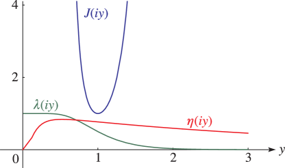
… ►For the functions $J_{\nu }\left(z\right)$, $Y_{\nu }\left(z\right)$, $H_{\nu }^{(1)}\left(z\right)$, $H_{\nu }^{(2)}\left(z\right)$, $I_{\nu }\left(z\right)$, and $K_{\nu }\left(z\right)$ see §§10.2(ii), 10.25(ii). ►The functions treated in this chapter are the Struve functions ${𝐇}_{\nu }\left(z\right)$ and ${𝐊}_{\nu }\left(z\right)$, the modified Struve functions ${𝐋}_{\nu }\left(z\right)$ and ${𝐌}_{\nu }\left(z\right)$, the Lommel functions $s_{\mu ,\nu }\left(z\right)$ and $S_{\mu ,\nu }\left(z\right)$, the Anger function ${𝐉}_{\nu }\left(z\right)$, the Weber function ${𝐄}_{\nu }\left(z\right)$, and the associated Anger–Weber function ${𝐀}_{\nu }\left(z\right)$.

26: 23.16 Graphics

… ►See Figures 23.16.1–23.16.3 for the modular functions $\lambda$, $J$, and $\eta$. … ►

►►

Figure 23.16.1: Modular functions $\lambda \left(\mathrm{i}y\right)$, $J\left(\mathrm{i}y\right)$, $\eta \left(\mathrm{i}y\right)$ for $0\le y\le 3$. … Magnify

… ►

►

►

Figure 23.16.3: Dedekind’s eta function $\eta \left(x+\mathrm{i}y\right)$ for $-0.0625\le x\le 0.0625$, $0.0001\le y\le 0.07$. Magnify 3D Help

27: 10.7 Limiting Forms

… ►

10.7.2 $$H_0^{(1)}\left(z\right)\sim -H_0^{(2)}\left(z\right)\sim (2\mathrm{i}/\pi )\ln z,$$

ⓘ

Symbols:

$H_{\nu }^{(1)}\left(z\right)$: Bessel function of the third kind (or Hankel function), $H_{\nu }^{(2)}\left(z\right)$: Bessel function of the third kind (or Hankel function), $\sim$: asymptotic equality, $\pi$: the ratio of the circumference of a circle to its diameter, $\mathrm{i}$: imaginary unit, $\ln z$: principal branch of logarithm function and $z$: complex variable

A&S Ref:

9.1.8

Referenced by:

§10.7(i)

Permalink:

http://dlmf.nist.gov/10.7.E2

Encodings:

pMML, png, TeX

See also:

Annotations for §10.7(i), §10.7 and Ch.10

… ►

10.7.7 $$H_{\nu }^{(1)}\left(z\right)\sim -H_{\nu }^{(2)}\left(z\right)\sim -(\mathrm{i}/\pi )\mathrm{\Gamma }\left(\nu \right){(\frac{1}{2}z)}^{-\nu },$$ $\mathrm{\Re }\nu >0$.

ⓘ

Symbols:

$\mathrm{\Gamma }\left(z\right)$: gamma function, $H_{\nu }^{(1)}\left(z\right)$: Bessel function of the third kind (or Hankel function), $H_{\nu }^{(2)}\left(z\right)$: Bessel function of the third kind (or Hankel function), $\sim$: asymptotic equality, $\pi$: the ratio of the circumference of a circle to its diameter, $\mathrm{i}$: imaginary unit, $\mathrm{\Re }$: real part, $z$: complex variable and $\nu$: complex parameter

Referenced by:

§10.7(i), §10.7(i)

Permalink:

http://dlmf.nist.gov/10.7.E7

Encodings:

pMML, png, TeX

See also:

Annotations for §10.7(i), §10.7 and Ch.10

►For $H_{-\nu }^{(1)}\left(z\right)$ and $H_{-\nu }^{(2)}\left(z\right)$ when $\mathrm{\Re }\nu >0$ combine (10.4.6) and (10.7.7). For $H_{\mathrm{i}\nu }^{(1)}\left(z\right)$ and $H_{\mathrm{i}\nu }^{(2)}\left(z\right)$ when $\nu \in ℝ$ and $\nu \ne 0$ combine (10.4.3), (10.7.3), and (10.7.6). … ►For the corresponding results for $H_{\nu }^{(1)}\left(z\right)$ and $H_{\nu }^{(2)}\left(z\right)$ see (10.2.5) and (10.2.6).

28: 10.16 Relations to Other Functions

… ►

$$H_{\frac{1}{2}}^{(1)}\left(z\right)=-\mathrm{i}{H}_{-\frac{1}{2}}^{(1)}\left(z\right)=-\mathrm{i}{\left(\frac{2}{\pi z}\right)}^{\frac{1}{2}}{\mathrm{e}}^{\mathrm{i}z},$$

►

$$H_{\frac{1}{2}}^{(2)}\left(z\right)=\mathrm{i}{H}_{-\frac{1}{2}}^{(2)}\left(z\right)=\mathrm{i}{\left(\frac{2}{\pi z}\right)}^{\frac{1}{2}}{\mathrm{e}}^{-\mathrm{i}z}.$$

… ►

10.16.6 $$\begin{array}{c}{H}_{\nu }^{(1)}\left(z\right)\\ H_{\nu }^{(2)}\left(z\right)\end{array}\}=\mp 2{\pi }^{-\frac{1}{2}}\mathrm{i}{\mathrm{e}}^{\mp \nu \pi \mathrm{i}}{(2z)}^{\nu }{\mathrm{e}}^{\pm \mathrm{i}z}U(\nu +\frac{1}{2},2\nu +1,\mp 2\mathrm{i}z).$$

ⓘ

Symbols:

$H_{\nu }^{(1)}\left(z\right)$: Bessel function of the third kind (or Hankel function), $H_{\nu }^{(2)}\left(z\right)$: Bessel function of the third kind (or Hankel function), $U(a,b,z)$: Kummer confluent hypergeometric function, $\pi$: the ratio of the circumference of a circle to its diameter, $\mathrm{e}$: base of natural logarithm, $\mathrm{i}$: imaginary unit, $z$: complex variable and $\nu$: complex parameter

Referenced by:

§10.16, §10.17(v)

Permalink:

http://dlmf.nist.gov/10.16.E6

Encodings:

pMML, png, TeX

See also:

Annotations for §10.16, §10.16 and Ch.10

… ►

10.16.8 $$\begin{array}{c}{H}_{\nu }^{(1)}\left(z\right)\\ H_{\nu }^{(2)}\left(z\right)\end{array}\}={\mathrm{e}}^{\mp (2\nu +1)\pi \mathrm{i}/4}{\left(\frac{2}{\pi z}\right)}^{\frac{1}{2}}{W}_{0,\nu }\left(\mp 2\mathrm{i}z\right).$$

ⓘ

Symbols:

$H_{\nu }^{(1)}\left(z\right)$: Bessel function of the third kind (or Hankel function), $H_{\nu }^{(2)}\left(z\right)$: Bessel function of the third kind (or Hankel function), $W_{\kappa ,\mu }\left(z\right)$: Whittaker confluent hypergeometric function, $\pi$: the ratio of the circumference of a circle to its diameter, $\mathrm{e}$: base of natural logarithm, $\mathrm{i}$: imaginary unit, $z$: complex variable and $\nu$: complex parameter

Referenced by:

§10.16, §10.16

Permalink:

http://dlmf.nist.gov/10.16.E8

Encodings:

pMML, png, TeX

See also:

Annotations for §10.16, §10.16 and Ch.10

…

29: 25.16 Mathematical Applications

… ►Euler sums have the form …where $H_n$ is given by (25.11.33). … ►For integer $s$ ($\ge 2$), $H\left(s\right)$ can be evaluated in terms of the zeta function: … ► $H\left(s\right)$ is the special case $H(s,1)$ of the function …when both $H(s,z)$ and $H(z,s)$ are finite. …

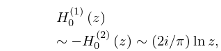
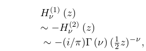
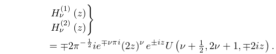
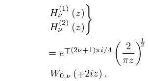
30: 33.15 Graphics

… ►

§33.15(i) Line Graphs of the Coulomb Functions $f(ϵ,\mathrm{\ell };r)$ and $h(ϵ,\mathrm{\ell };r)$

►

►►

Figure 33.15.1: $f(ϵ,\mathrm{\ell };r),h(ϵ,\mathrm{\ell };r)$ with $\mathrm{\ell }=0,ϵ=4$. Magnify

►

►►

Figure 33.15.2: $f(ϵ,\mathrm{\ell };r),h(ϵ,\mathrm{\ell };r)$ with $\mathrm{\ell }=1,ϵ=4$. Magnify

… ►

§33.15(ii) Surfaces of the Coulomb Functions $f(ϵ,\mathrm{\ell };r)$, $h(ϵ,\mathrm{\ell };r)$, $s(ϵ,\mathrm{\ell };r)$, and $c(ϵ,\mathrm{\ell };r)$

… ►

►

►

Figure 33.15.7: $h(ϵ,\mathrm{\ell };r)$ with . Magnify 3D Help

…