金肯职业技术学院毕业证制作【言正 微aptao168】0oB4ifw

SearchAdvancedHelp

(0.004 seconds)

21—30 of 697 matching pages

21: 31.5 Solutions Analytic at Three Singularities: Heun Polynomials

… ►Let $\alpha =-n$, $n=0,1,2,\mathrm{\dots }$, and $q_{n,m}$, $m=0,1,\mathrm{\dots },n$, be the eigenvalues of the tridiagonal matrix ►

31.5.1

ⓘ

Symbols:

$\gamma$: real or complex parameter, $n$: nonnegative integer, $a$: complex parameter, $P_j$: coefficient, $Q_j$: coefficient and $R_j$: coefficient

Permalink:

http://dlmf.nist.gov/31.5.E1

Encodings:

pMML, png, TeX

See also:

Annotations for §31.5 and Ch.31

… ►is a polynomial of degree $n$, and hence a solution of (31.2.1) that is analytic at all three finite singularities $0,1,a$. …

22: 10.75 Tables

… ►

Achenbach (1986) tabulates $J_0\left(x\right)$, $J_1\left(x\right)$, $Y_0\left(x\right)$, $Y_1\left(x\right)$, $x=0(.1)8$, 20D or 18–20S.

… ►

Abramowitz and Stegun (1964, Chapter 11) tabulates ${\int }_0^x{J}_0\left(t\right)dt$, ${\int }_0^x{Y}_0\left(t\right)dt$, $x=0(.1)10$, 10D; ${\int }_0^x{t}^{-1}(1-J_0\left(t\right))dt$, ${\int }_x^{\mathrm{\infty }}{t}^{-1}{Y}_0\left(t\right)dt$, $x=0(.1)5$, 8D.

►

Zhang and Jin (1996, p. 270) tabulates ${\int }_0^x{J}_0\left(t\right)dt$, ${\int }_0^x{t}^{-1}(1-J_0\left(t\right))dt$, ${\int }_0^x{Y}_0\left(t\right)dt$, ${\int }_x^{\mathrm{\infty }}{t}^{-1}{Y}_0\left(t\right)dt$, $x=0(.1)1(.5)20$, 8D.

… ►

Achenbach (1986) tabulates $I_0\left(x\right)$, $I_1\left(x\right)$, $K_0\left(x\right)$, $K_1\left(x\right)$, $x=0(.1)8$, 19D or 19–21S.

… ►

Abramowitz and Stegun (1964, Chapter 11) tabulates ${\mathrm{e}}^{-x}{\int }_0^x{I}_0\left(t\right)dt$, ${\mathrm{e}}^x{\int }_x^{\mathrm{\infty }}{K}_0\left(t\right)dt$, $x=0(.1)10$, 7D; ${\mathrm{e}}^{-x}{\int }_0^x{t}^{-1}(I_0\left(t\right)-1)dt$, $x{\mathrm{e}}^x{\int }_x^{\mathrm{\infty }}{t}^{-1}{K}_0\left(t\right)dt$, $x=0(.1)5$, 6D.

…

23: 8.26 Tables

… ►

Pagurova (1963) tabulates $P(a,x)$ and $Q(a,x)$ (with different notation) for $a=0(.05)3$, $x=0(.05)1$ to 7D.

►

Pearson (1965) tabulates the function $I(u,p)$ ($=P(p+1,u)$) for $p=-1(.05)0(.1)5(.2)50$, $u=0(.1)u_p$ to 7D, where $I(u,u_p)$ rounds off to 1 to 7D; also $I(u,p)$ for $p=-0.75(.01)-1$, $u=0(.1)6$ to 5D.

►

Zhang and Jin (1996, Table 3.8) tabulates $\gamma (a,x)$ for $a=0.5,1,3,5,10,25,50,100$, $x=0(.1)1(1)3,5(5)30,50,100$ to 8D or 8S.

… ►

Abramowitz and Stegun (1964, pp. 245–248) tabulates $E_n\left(x\right)$ for $n=2,3,4,10,20$, $x=0(.01)2$ to 7D; also $(x+n){\mathrm{e}}^x{E}_n\left(x\right)$ for $n=2,3,4,10,20$, $x^{-1}=0(.01)0.1(.05)0.5$ to 6S.

… ►

Pagurova (1961) tabulates $E_n\left(x\right)$ for $n=0(1)20$, $x=0(.01)2(.1)10$ to 4-9S; ${\mathrm{e}}^x{E}_n\left(x\right)$ for $n=2(1)10$, $x=10(.1)20$ to 7D; ${\mathrm{e}}^x{E}_p\left(x\right)$ for $p=0(.1)1$, $x=0.01(.01)7(.05)12(.1)20$ to 7S or 7D.

…

24: 22.5 Special Values

… ►For example, at $z=K+\mathrm{i}{K}^{\prime }$, $\mathrm{sn}(z,k)=1/k$, $d\mathrm{sn}(z,k)/dz=0$. … ►

§22.5(ii) Limiting Values of $k$

►If $k\to 0+$, then $K\to \pi /2$ and $K^{\prime }\to \mathrm{\infty }$; if $k\to 1-$, then $K\to \mathrm{\infty }$ and $K^{\prime }\to \pi /2$. … ►Expansions for $K,K^{\prime }$ as $k\to 0$ or $1$ are given in §§19.5, 19.12. … ►

25: 21.4 Graphics

… ►This Riemann matrix originates from the Riemann surface represented by the algebraic curve ${\mu }^3-{\lambda }^7+2{\lambda }^3\mu =0$; compare §21.7(i). ►

…

Figure 21.4.1: $\widehat{\theta }\left(𝐳\right|𝛀)$ parametrized by (21.4.1). The surface plots are of $\widehat{\theta }\left(x+\mathrm{i}y,0\right|𝛀)$, $0\le x\le 1$, $0\le y\le 5$ (suffix 1); $\widehat{\theta }\left(x,y\right|𝛀)$, $0\le x\le 1$, $0\le y\le 1$ (suffix 2); $\widehat{\theta }\left(\mathrm{i}x,\mathrm{i}y\right|𝛀)$, $0\le x\le 5$, $0\le y\le 5$ (suffix 3). …

… ►

►

►

Figure 21.4.2: $\mathrm{\Re }\widehat{\theta }\left(x+\mathrm{i}y,0\right|{𝛀}_1)$, $0\le x\le 1$, $0\le y\le 5$. … Magnify 3D Help

►

►

►

Figure 21.4.3: $\left|\widehat{\theta }\left(x+\mathrm{i}y,0\right|{𝛀}_1)\right|$, $0\le x\le 1$, $0\le y\le 2$. Magnify 3D Help

… ►

►

►

Figure 21.4.5: The real part of a genus 3 scaled Riemann theta function: $\mathrm{\Re }\widehat{\theta }\left(x+\mathrm{i}y,0,0\right|{𝛀}_2)$, $0\le x\le 1$, $0\le y\le 3$. … Magnify 3D Help

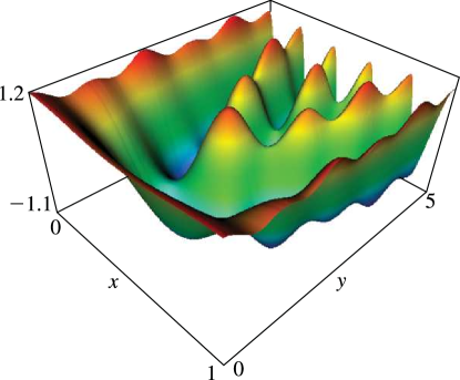
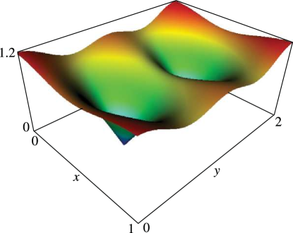
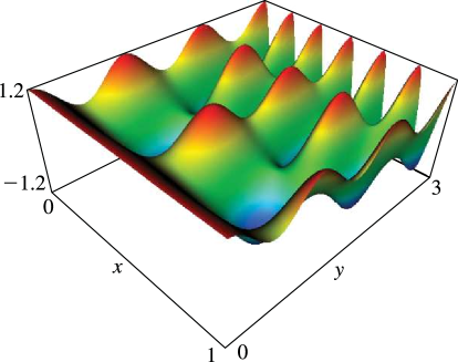
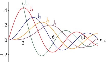
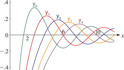
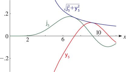
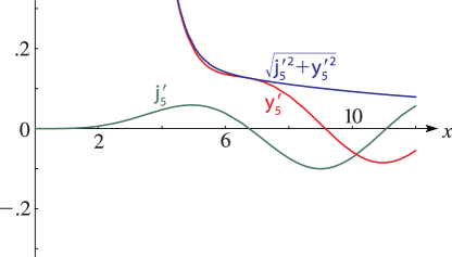
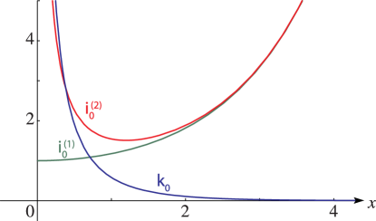
26: 10.48 Graphs

… ►

►►

Figure 10.48.1: ${𝗃}_n\left(x\right)$, $n=0(1)4$, $0\le x\le 12$. Magnify

►

►►

Figure 10.48.2: ${𝗒}_n\left(x\right)$, $n=0(1)4$, . Magnify

►

►►

Figure 10.48.3: ${𝗃}_5\left(x\right)$, ${𝗒}_5\left(x\right)$, $\sqrt{{𝗃}_5^2\left(x\right)+{𝗒}_5^2\left(x\right)}$, $0\le x\le 12$. Magnify

►

►►

Figure 10.48.4: ${𝗃}_5^{\prime }\left(x\right)$, ${𝗒}_5^{\prime }\left(x\right)$, $\sqrt{𝗃_5^{\prime }{}_{}{}^2\left(x\right)+𝗒_5^{\prime }{}_{}{}^2\left(x\right)}$, $0\le x\le 12$. Magnify

►

►►

Figure 10.48.5: ${𝗂}_0^{(1)}\left(x\right)$, ${𝗂}_0^{(2)}\left(x\right)$, ${𝗄}_0\left(x\right)$, $0\le x\le 4$. Magnify

…

27: 17.5 ${}_0{}^{}\varphi _0^{},{}_1{}^{}\varphi _0^{},{}_1{}^{}\varphi _1^{}$ Functions

§17.5 ${}_0{}^{}\varphi _0^{},{}_1{}^{}\varphi _0^{},{}_1{}^{}\varphi _1^{}$ Functions

… ►

17.5.1 $${}_0{}^{}\varphi _0^{}(-;-;q,z)=\sum _{n=0}^{\mathrm{\infty }}\frac{{(-1)}^n{q}^{\left(\genfrac{}{}{0.0pt}{}{n}{2}\right)}{z}^n}{{(q;q)}_n}={(z;q)}_{\mathrm{\infty }};$$

ⓘ

Symbols:

$\left(\genfrac{}{}{0.0pt}{}{m}{n}\right)$: binomial coefficient, ${(a;q)}_n$: $q$-Pochhammer symbol (or $q$-shifted factorial), ${}_{r+1}{}^{}\varphi _s^{}(a_0,\mathrm{\dots },a_r;b_1,\mathrm{\dots },b_s;q,z)$ or ${}_{r+1}{}^{}\varphi _s^{}(\genfrac{}{}{0pt}{}{a_0,\mathrm{\dots },a_r}{b_1,\mathrm{\dots },b_s};q,z)$: basic hypergeometric (or $q$-hypergeometric) function, $q$: complex base, $n$: nonnegative integer and $z$: complex variable

Referenced by:

§17.2(iii), Erratum (V1.1.11) for Equation (17.5.1)

Permalink:

http://dlmf.nist.gov/17.5.E1

Encodings:

pMML, png, TeX

Correction (effective with 1.1.11):

The constraint is not necessary and was removed.

See also:

Annotations for §17.5, §17.5 and Ch.17

… ►

17.5.2 $${}_1{}^{}\varphi _0^{}(a;-;q,z)=\frac{{(az;q)}_{\mathrm{\infty }}}{{(z;q)}_{\mathrm{\infty }}},$$ ;

ⓘ

Symbols:

${(a;q)}_n$: $q$-Pochhammer symbol (or $q$-shifted factorial), ${}_{r+1}{}^{}\varphi _s^{}(a_0,\mathrm{\dots },a_r;b_1,\mathrm{\dots },b_s;q,z)$ or ${}_{r+1}{}^{}\varphi _s^{}(\genfrac{}{}{0pt}{}{a_0,\mathrm{\dots },a_r}{b_1,\mathrm{\dots },b_s};q,z)$: basic hypergeometric (or $q$-hypergeometric) function, $q$: complex base and $z$: complex variable

Permalink:

http://dlmf.nist.gov/17.5.E2

Encodings:

pMML, png, TeX

See also:

Annotations for §17.5, §17.5 and Ch.17

… ►

17.5.3 $${}_1{}^{}\varphi _0^{}(q^{-n};-;q,z)={(z{q}^{-n};q)}_n.$$

ⓘ

Symbols:

${(a;q)}_n$: $q$-Pochhammer symbol (or $q$-shifted factorial), ${}_{r+1}{}^{}\varphi _s^{}(a_0,\mathrm{\dots },a_r;b_1,\mathrm{\dots },b_s;q,z)$ or ${}_{r+1}{}^{}\varphi _s^{}(\genfrac{}{}{0pt}{}{a_0,\mathrm{\dots },a_r}{b_1,\mathrm{\dots },b_s};q,z)$: basic hypergeometric (or $q$-hypergeometric) function, $q$: complex base, $n$: nonnegative integer and $z$: complex variable

Permalink:

http://dlmf.nist.gov/17.5.E3

Encodings:

pMML, png, TeX

See also:

Annotations for §17.5, §17.5 and Ch.17

… ►

17.5.4 $${}_1{}^{}\varphi _0^{}(0;-;q,z)=\sum _{n=0}^{\mathrm{\infty }}\frac{z^n}{{(q;q)}_n}=\frac{1}{{(z;q)}_{\mathrm{\infty }}},$$ ;

ⓘ

Symbols:

${(a;q)}_n$: $q$-Pochhammer symbol (or $q$-shifted factorial), ${}_{r+1}{}^{}\varphi _s^{}(a_0,\mathrm{\dots },a_r;b_1,\mathrm{\dots },b_s;q,z)$ or ${}_{r+1}{}^{}\varphi _s^{}(\genfrac{}{}{0pt}{}{a_0,\mathrm{\dots },a_r}{b_1,\mathrm{\dots },b_s};q,z)$: basic hypergeometric (or $q$-hypergeometric) function, $q$: complex base, $n$: nonnegative integer and $z$: complex variable

Referenced by:

§17.2(iii)

Permalink:

http://dlmf.nist.gov/17.5.E4

Encodings:

pMML, png, TeX

See also:

Annotations for §17.5, §17.5 and Ch.17

…

28: 36.15 Methods of Computation

… ►Close to the origin $𝐱=\mathrm{𝟎}$ of parameter space, the series in §36.8 can be used. … ►Close to the bifurcation set but far from $𝐱=\mathrm{𝟎}$, the uniform asymptotic approximations of §36.12 can be used. …

29: 19.22 Quadratic Transformations

… ►The AGM, $M(a_0,g_0)$, of two positive numbers $a_0$ and $g_0$ is defined in §19.8(i). …$Q_n$ has the same sign as $a_0-g_0$ for $n\ge 1$. …where $p_0>0$ and …As $n\to \mathrm{\infty }$, $p_n$ and ${\epsilon }_n$ converge quadratically to $M(a_0,g_0)$ and 0, respectively, and $Q_n$ converges to 0 faster than quadratically. … ►If $p=x$ or $p=y$, then (19.22.20) reduces to $0=0$ by (19.20.13), and if $z=x$ or $z=y$ then (19.22.19) reduces to $0=0$ by (19.20.20) and (19.22.22). …

30: 7.23 Tables

… ►

Abramowitz and Stegun (1964, Chapter 7) includes $\mathrm{erf}x$, $(2/\sqrt{\pi }){\mathrm{e}}^{-x^2}$, $x\in [0,2]$, 10D; $(2/\sqrt{\pi }){\mathrm{e}}^{-x^2}$, $x\in [2,10]$, 8S; $x{\mathrm{e}}^{x^2}\mathrm{erfc}x$, $x^{-2}\in [0,0.25]$, 7D; $2^n\mathrm{\Gamma }\left(\frac{1}{2}n+1\right){\mathrm{i}}^n\mathrm{erfc}\left(x\right)$, $n=1(1)6,10,11$, $x\in [0,5]$, 6S; $F\left(x\right)$, $x\in [0,2]$, 10D; $xF\left(x\right)$, $x^{-2}\in [0,0.25]$, 9D; $C\left(x\right)$, $S\left(x\right)$, $x\in [0,5]$, 7D; $\mathrm{f}\left(x\right)$, $\mathrm{g}\left(x\right)$, $x\in [0,1]$, $x^{-1}\in [0,1]$, 15D.

►

Abramowitz and Stegun (1964, Table 27.6) includes the Goodwin–Staton integral $G\left(x\right)$, $x=1(.1)3(.5)8$, 4D; also $G\left(x\right)+\ln x$, $x=0(.05)1$, 4D.

►

Finn and Mugglestone (1965) includes the Voigt function $H(a,u)$, $u\in [0,22]$, $a\in [0,1]$, 6S.

►

Zhang and Jin (1996, pp. 637, 639) includes $(2/\sqrt{\pi }){\mathrm{e}}^{-x^2}$, $\mathrm{erf}x$, $x=0(.02)1(.04)3$, 8D; $C\left(x\right)$, $S\left(x\right)$, $x=0(.2)10(2)100(100)500$, 8D.

… ►

Abramowitz and Stegun (1964, Chapter 7) includes $w\left(z\right)$, $x=0(.1)3.9$, $y=0(.1)3$, 6D.

…