DLMF: Untitled Document

… ► ►►►

	Open Source								With Book	Commercial
…
19.39(ii) $K\left(k\right)$ , $E\left(k\right)$ , $0\leq k^{2}\leq 1$	✓	✓	✓	✓	✓	✓	✓	✓		✓	✓	✓	✓
…

… ►

Open Source Collections and Systems.

These are collections of software (e.g. libraries) or interactive systems of a somewhat broad scope. Contents may be adapted from research software or may be contributed by project participants who donate their services to the project. The software is made freely available to the public, typically in source code form. While formal support of the collection may not be provided by its developers, within active projects there is often a core group who donate time to consider bug reports and make updates to the collection.

…

… ►

•

Abramowitz and Stegun (1964, Chapter 14) tabulates $F_{0}\left(\eta,\rho\right)$ , $G_{0}\left(\eta,\rho\right)$ , $F_{0}'\left(\eta,\rho\right)$ , and $G_{0}'\left(\eta,\rho\right)$ for $\eta=0.5(.5)20$ and $\rho=1(1)20$ , 5S; $C_{0}\left(\eta\right)$ for $\eta=0(.05)3$ , 6S.

►

•

Curtis (1964a) tabulates $P_{\ell}(\epsilon,r)$ , $Q_{\ell}(\epsilon,r)$ (§33.1), and related functions for $\ell=0,1,2$ and $\epsilon=-2(.2)2$ , with $x=0(.1)4$ for $\epsilon<0$ and $x=0(.1)10$ for $\epsilon\geq 0$ ; 6D.

…

… ►The set

\mathfrak{S}_{n}

(§26.13) can be identified with the set of

n\times n

matrices of 0’s and 1’s with exactly one 1 in each row and column. The permutation

\sigma

corresponds to the matrix in which there is a 1 at the intersection of row

j

with column

\sigma(j)

, and 0’s in all other positions. … ►Define

r_{0}(B)=1

. … ►The Ferrers board of shape

(b_{1},b_{2},\ldots,b_{n})

,

0\leq b_{1}\leq b_{2}\leq\cdots\leq b_{n}

, is the set

B=\{(j,k)\>|\>1\leq j\leq n,1\leq k\leq b_{j}\}

. …If

B

is the Ferrers board of shape

(0,1,2,\ldots,n-1)

, then …

… ►

B_{2n+1}=0

,

►

(-1)^{n+1}B_{2n}>0

,

n=1,2,\dots

.

… ►

E_{2n+1}=0

,

►

(-1)^{n}E_{2n}>0

.

… ►

\widetilde{E}_{n}\left(x\right)=E_{n}\left(x\right)

,

0\leq x<1

,

…

… ►

•

Abramowitz and Stegun (1964, Chapter 12) tabulates $\mathbf{H}_{n}\left(x\right)$ , $\mathbf{H}_{n}\left(x\right)-Y_{n}\left(x\right)$ , and $I_{n}\left(x\right)-\mathbf{L}_{n}\left(x\right)$ for $n=0,1$ and $x=0(.1)5$ , $x^{-1}=0(.01)0.2$ to 6D or 7D.

►

•

Agrest et al. (1982) tabulates $\mathbf{H}_{n}\left(x\right)$ and $e^{-x}\mathbf{L}_{n}\left(x\right)$ for $n=0,1$ and $x=0(.001)5(.005)15(.01)100$ to 11D.

… ►

•

Abramowitz and Stegun (1964, Chapter 12) tabulates $\int_{0}^{x}(I_{0}\left(t\right)-\mathbf{L}_{0}\left(t\right))\,\mathrm{d}t$ and $(2/\pi)\int_{x}^{\infty}t^{-1}\mathbf{H}_{0}\left(t\right)\,\mathrm{d}t$ for $x=0(.1)5$ to 5D or 7D; $\int_{0}^{x}(\mathbf{H}_{0}\left(t\right)-Y_{0}\left(t\right))\,\mathrm{d}t-(2% /\pi)\ln x$ , $\int_{0}^{x}(I_{0}\left(t\right)-\mathbf{L}_{0}\left(t\right))\,\mathrm{d}t-(2% /\pi)\ln x$ , and $\int_{x}^{\infty}t^{-1}(\mathbf{H}_{0}\left(t\right)-Y_{0}\left(t\right))\,% \mathrm{d}t$ for $x^{-1}=0(.01)0.2$ to 6D.

►

•

Agrest et al. (1982) tabulates $\int_{0}^{x}\mathbf{H}_{0}\left(t\right)\,\mathrm{d}t$ and $e^{-x}\int_{0}^{x}\mathbf{L}_{0}\left(t\right)\,\mathrm{d}t$ for $x=0(.001)5(.005)15(.01)100$ to 11D.

… ►

•

Agrest and Maksimov (1971, Chapter 11) defines incomplete Struve, Anger, and Weber functions and includes tables of an incomplete Struve function $\mathbf{H}_{n}\left(x,\alpha\right)$ for $n=0,1$ , $x=0(.2)10$ , and $\alpha=0(.2)1.4,\tfrac{1}{2}\pi$ , together with surface plots.

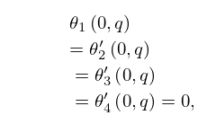
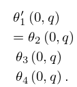
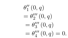
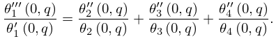
§20.4 Values at $z$ = 0

… ►

20.4.1

\theta_{1}\left(0,q\right)=\theta_{2}'\left(0,q\right)=\theta_{3}'\left(0,q% \right)=\theta_{4}'\left(0,q\right)=0,

ⓘ

Symbols:: $\theta_{\NVar{j}}\left(\NVar{z},\NVar{q}\right)$ : theta function and $q$ : nome
Permalink:: http://dlmf.nist.gov/20.4.E1
Encodings:: pMML, png, TeX
See also:: Annotations for §20.4(i), §20.4 and Ch.20

… ►

20.4.6

\theta_{1}'\left(0,q\right)=\theta_{2}\left(0,q\right)\theta_{3}\left(0,q% \right)\theta_{4}\left(0,q\right).

ⓘ

Symbols:: $\theta_{\NVar{j}}\left(\NVar{z},\NVar{q}\right)$ : theta function and $q$ : nome
A&S Ref:: 16.28.6
Referenced by:: §20.9(i)
Permalink:: http://dlmf.nist.gov/20.4.E6
Encodings:: pMML, png, TeX
See also:: Annotations for §20.4(i), §20.4(i), §20.4 and Ch.20

… ►

20.4.7

\theta_{1}''\left(0,q\right)=\theta_{2}'''\left(0,q\right)=\theta_{3}'''\left(% 0,q\right)=\theta_{4}'''\left(0,q\right)=0.

ⓘ

Symbols:: $\theta_{\NVar{j}}\left(\NVar{z},\NVar{q}\right)$ : theta function and $q$ : nome
Permalink:: http://dlmf.nist.gov/20.4.E7
Encodings:: pMML, png, TeX
See also:: Annotations for §20.4(ii), §20.4 and Ch.20

… ►

20.4.12

\frac{\theta_{1}'''\left(0,q\right)}{\theta_{1}'\left(0,q\right)}=\frac{\theta% _{2}''\left(0,q\right)}{\theta_{2}\left(0,q\right)}+\frac{\theta_{3}''\left(0,% q\right)}{\theta_{3}\left(0,q\right)}+\frac{\theta_{4}''\left(0,q\right)}{% \theta_{4}\left(0,q\right)}.

ⓘ

Symbols:: $\theta_{\NVar{j}}\left(\NVar{z},\NVar{q}\right)$ : theta function and $q$ : nome
Permalink:: http://dlmf.nist.gov/20.4.E12
Encodings:: pMML, png, TeX
See also:: Annotations for §20.4(ii), §20.4 and Ch.20

… ►

Table 4.31.1: Hyperbolic functions: values at multiples of

\tfrac{1}{2}\pi i

.

► ►►►►

$z$	0	$\frac{1}{2}\pi\mathrm{i}$	$\pi\mathrm{i}$	$\frac{3}{2}\pi\mathrm{i}$	$\infty$
…
$\cosh z$	$1$	$0$	$-1$	$0$	$\infty$
…
$\coth z$	$\infty$	$0$	$\infty$	$0$	$1$

► ►

4.31.1

\lim_{z\to 0}\frac{\sinh z}{z}=1,

ⓘ

Symbols:: $\sinh\NVar{z}$ : hyperbolic sine function and $z$ : complex variable
Permalink:: http://dlmf.nist.gov/4.31.E1
Encodings:: pMML, png, TeX
See also:: Annotations for §4.31 and Ch.4

►

4.31.2

\lim_{z\to 0}\frac{\tanh z}{z}=1,

ⓘ

Symbols:: $\tanh\NVar{z}$ : hyperbolic tangent function and $z$ : complex variable
Permalink:: http://dlmf.nist.gov/4.31.E2
Encodings:: pMML, png, TeX
See also:: Annotations for §4.31 and Ch.4

►

4.31.3

\lim_{z\to 0}\frac{\cosh z-1}{z^{2}}=\frac{1}{2}.

ⓘ

Symbols:: $\cosh\NVar{z}$ : hyperbolic cosine function and $z$ : complex variable
Permalink:: http://dlmf.nist.gov/4.31.E3
Encodings:: pMML, png, TeX
See also:: Annotations for §4.31 and Ch.4

… ►

32.4.10

zu_{0}^{\prime}=\theta_{\infty}u_{0}-zv_{0}v_{1},

ⓘ

Symbols:: $z$ : real and $\theta_{\infty}$ : constant
Referenced by:: §32.4(iv)
Permalink:: http://dlmf.nist.gov/32.4.E10
Encodings:: pMML, png, TeX
See also:: Annotations for §32.4(iv), §32.4 and Ch.32

… ►

32.4.12

zv_{0}^{\prime}=2v_{0}u_{1}v_{1}+v_{0}+(u_{0}(2v_{0}-z)/v_{1}),

ⓘ

Symbols:: $z$ : real
Permalink:: http://dlmf.nist.gov/32.4.E12
Encodings:: pMML, png, TeX
See also:: Annotations for §32.4(iv), §32.4 and Ch.32

… ►If

w=-u_{0}/(v_{0}v_{1})

, then …where ►

32.4.16

\theta_{0}=\frac{4v_{0}}{z}\left(\theta_{\infty}\left(1-\frac{z}{4v_{0}}\right% )+\frac{z-2v_{0}}{2v_{0}v_{1}}u_{0}+u_{1}v_{1}\right).

ⓘ

Symbols:: $z$ : real, $\theta_{\infty}$ : constant and $\theta_{0}$
Permalink:: http://dlmf.nist.gov/32.4.E16
Encodings:: pMML, png, TeX
See also:: Annotations for §32.4(iv), §32.4 and Ch.32

…

… ►

•

Abramowitz and Stegun (1964, Chapter 8) tabulates $\mathsf{P}_{n}\left(x\right)$ for $n=0(1)3,9,10$ , $x=0(.01)1$ , 5–8D; $\mathsf{P}_{n}'\left(x\right)$ for $n=1(1)4,9,10$ , $x=0(.01)1$ , 5–7D; $\mathsf{Q}_{n}\left(x\right)$ and $\mathsf{Q}_{n}'\left(x\right)$ for $n=0(1)3,9,10$ , $x=0(.01)1$ , 6–8D; $P_{n}\left(x\right)$ and $P_{n}'\left(x\right)$ for $n=0(1)5,9,10$ , $x=1(.2)10$ , 6S; $Q_{n}\left(x\right)$ and $Q_{n}'\left(x\right)$ for $n=0(1)3,9,10$ , $x=1(.2)10$ , 6S. (Here primes denote derivatives with respect to $x$ .)

►

•

Zhang and Jin (1996, Chapter 4) tabulates $\mathsf{P}_{n}\left(x\right)$ for $n=2(1)5,10$ , $x=0(.1)1$ , 7D; $\mathsf{P}_{n}\left(\cos\theta\right)$ for $n=1(1)4,10$ , $\theta=0(5^{\circ})90^{\circ}$ , 8D; $\mathsf{Q}_{n}\left(x\right)$ for $n=0(1)2,10$ , $x=0(.1)0.9$ , 8S; $\mathsf{Q}_{n}\left(\cos\theta\right)$ for $n=0(1)3,10$ , $\theta=0(5^{\circ})90^{\circ}$ , 8D; $\mathsf{P}^{m}_{n}\left(x\right)$ for $m=1(1)4$ , $n-m=0(1)2$ , $n=10$ , $x=0,0.5$ , 8S; $\mathsf{Q}^{m}_{n}\left(x\right)$ for $m=1(1)4$ , $n=0(1)2,10$ , 8S; $\mathsf{P}^{m}_{\nu}\left(\cos\theta\right)$ for $m=0(1)3$ , $\nu=0(.25)5$ , $\theta=0(15^{\circ})90^{\circ}$ , 5D; $P_{n}\left(x\right)$ for $n=2(1)5,10$ , $x=1(1)10$ , 7S; $Q_{n}\left(x\right)$ for $n=0(1)2,10$ , $x=2(1)10$ , 8S. Corresponding values of the derivative of each function are also included, as are 6D values of the first 5 $\nu$ -zeros of $\mathsf{P}^{m}_{\nu}\left(\cos\theta\right)$ and of its derivative for $m=0(1)4$ , $\theta=10^{\circ},30^{\circ},150^{\circ}$ .

►

•

Belousov (1962) tabulates $\mathsf{P}^{m}_{n}\left(\cos\theta\right)$ (normalized) for $m=0(1)36$ , $n-m=0(1)56$ , $\theta=0(2.5^{\circ})90^{\circ}$ , 6D.

►

•

Žurina and Karmazina (1964, 1965) tabulate the conical functions $\mathsf{P}_{-\frac{1}{2}+\mathrm{i}\tau}\left(x\right)$ for $\tau=0(.01)50$ , $x=-0.9(.1)0.9$ , 7S; $P_{-\frac{1}{2}+\mathrm{i}\tau}\left(x\right)$ for $\tau=0(.01)50$ , $x=1.1(.1)2(.2)5(.5)10(10)60$ , 7D. Auxiliary tables are included to facilitate computation for larger values of $\tau$ when $-1<x<1$ .

►

•

Žurina and Karmazina (1963) tabulates the conical functions $\mathsf{P}^{1}_{-\frac{1}{2}+\mathrm{i}\tau}\left(x\right)$ for $\tau=0(.01)25$ , $x=-0.9(.1)0.9$ , 7S; $P^{1}_{-\frac{1}{2}+\mathrm{i}\tau}\left(x\right)$ for $\tau=0(.01)25$ , $x=1.1(.1)2(.2)5(.5)10(10)60$ , 7S. Auxiliary tables are included to assist computation for larger values of $\tau$ when $-1<x<1$ .

…

… ►

15.15.1

\mathbf{F}\left({a,b\atop c};\frac{1}{z}\right)=\left(1-\frac{z_{0}}{z}\right)% ^{-a}\sum_{s=0}^{\infty}\frac{{\left(a\right)_{s}}}{s!}\*\mathbf{F}\left({-s,b% \atop c};\frac{1}{z_{0}}\right)\left(1-\frac{z}{z_{0}}\right)^{-s}.

ⓘ

Symbols:: ${\left(\NVar{a}\right)_{\NVar{n}}}$ : Pochhammer’s symbol (or shifted factorial), $!$ : factorial (as in $n!$ ), $\mathbf{F}\left(\NVar{a},\NVar{b};\NVar{c};\NVar{z}\right)$ or $\mathbf{F}\left({\NVar{a},\NVar{b}\atop\NVar{c}};\NVar{z}\right)$ : $={{}_{2}{\mathbf{F}}_{1}}\left(\NVar{a},\NVar{b};\NVar{c};\NVar{z}\right)$ Olver’s hypergeometric function, $s$ : nonnegative integer, $z$ : complex variable, $a$ : real or complex parameter, $b$ : real or complex parameter and $c$ : real or complex parameter
Referenced by:: §15.19(i)
Permalink:: http://dlmf.nist.gov/15.15.E1
Encodings:: pMML, png, TeX
Correction (effective with 1.1.2):: The Pochhammer symbol now links to its definition.
See also:: Annotations for §15.15 and Ch.15

►Here

z_{0}

(

{\neq 0}

) is an arbitrary complex constant and the expansion converges when

|z-z_{0}|>\max(|z_{0}|,|z_{0}-1|)

. …

没有中专毕业证可以参加高职高考吗【somewhat微aptao168】0A1mFwg

1—10 of 697 matching pages

1: Software Index

2: 33.24 Tables

3: 26.15 Permutations: Matrix Notation

4: 24.2 Definitions and Generating Functions

5: 11.14 Tables

6: 20.4 Values at $z$ = 0

§20.4 Values at $z$ = 0

7: 4.31 Special Values and Limits

8: 32.4 Isomonodromy Problems

9: 14.33 Tables

10: 15.15 Sums

没有中专毕业证可以参加高职高考吗【somewhat微aptao168】0A1mFwg

1—10 of 697 matching pages

1: Software Index

2: 33.24 Tables

3: 26.15 Permutations: Matrix Notation

4: 24.2 Definitions and Generating Functions

5: 11.14 Tables

6: 20.4 Values at z = 0

§20.4 Values at z = 0

7: 4.31 Special Values and Limits

8: 32.4 Isomonodromy Problems

9: 14.33 Tables

10: 15.15 Sums

6: 20.4 Values at $z$ = 0

§20.4 Values at $z$ = 0