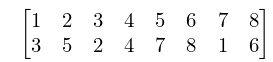
About the Project

Previous 10 matching pages Next 10 matching pages

怎么做假雅芳-斯特拉特福学院文凭毕业证【购证微kaa77788】5Tpe

♦ 21—30 of 286 matching pages ♦

(0.003 seconds)

21—30 of 286 matching pages

21: 15.3 Graphics

… ►

See accompanying text — Figure 15.3.1: $F\left(\tfrac{4}{3},\tfrac{9}{16};\tfrac{14}{5};x\right),-100\leq x\leq 1$ . Magnify

►

See accompanying text — Figure 15.3.2: $F\left(5,-10;1;x\right),-0.023\leq x\leq 1$ . Magnify

… ►

See accompanying text — Figure 15.3.4: $F\left(5,10;1;x\right),-1\leq x\leq 0.022$ . Magnify

… ►

See accompanying text — Figure 15.3.5: $F\left(\tfrac{4}{3},\tfrac{9}{16};\tfrac{14}{5};x+\mathrm{i}y\right),0\leq x% \leq 2,-0.5\leq y\leq 0.5$ . … Magnify 3D Help

►

See accompanying text — Figure 15.3.6: $F\left(-3,\frac{3}{5};u+\mathrm{i}v;\frac{1}{2}\right),-6\leq u\leq 2,-2\leq v\leq 2$ . … Magnify 3D Help

…

22: 26.13 Permutations: Cycle Notation

… ►

26.13.2

\begin{bmatrix}1&2&3&4&5&6&7&8\\ 3&5&2&4&7&8&1&6\end{bmatrix}

ⓘ

Referenced by:: §26.13, §26.13, §26.13
Permalink:: http://dlmf.nist.gov/26.13.E2
Encodings:: pMML, png, TeX
See also:: Annotations for §26.13 and Ch.26

►is

{\left(1,3,2,5,7\right)}{\left(4\right)}{\left(6,8\right)}

in cycle notation. …In consequence, (26.13.2) can also be written as

{\left(1,3,2,5,7\right)}{\left(6,8\right)}

. … ►For the example (26.13.2), this decomposition is given by

{\left(1,3,2,5,7\right)}{\left(6,8\right)}={\left(1,3\right)}{\left(2,3\right)% }{\left(2,5\right)}{\left(5,7\right)}{\left(6,8\right)}.

… ►Again, for the example (26.13.2) a minimal decomposition into adjacent transpositions is given by

{\left(1,3,2,5,7\right)}{\left(6,8\right)}={\left(2,3\right)}\*{\left(1,2% \right)}\*{\left(4,5\right)}{\left(3,4\right)}{\left(2,3\right)}{\left(3,4% \right)}{\left(4,5\right)}{\left(6,7\right)}{\left(5,6\right)}{\left(7,8\right% )}\*{\left(6,7\right)}

:

\mathop{\mathrm{inv}}({\left(1,3,2,5,7\right)}{\left(6,8\right)})=11

.

23: 25.20 Approximations

… ►

•

Cody et al. (1971) gives rational approximations for $\zeta\left(s\right)$ in the form of quotients of polynomials or quotients of Chebyshev series. The ranges covered are $0.5\leq s\leq 5$ , $5\leq s\leq 11$ , $11\leq s\leq 25$ , $25\leq s\leq 55$ . Precision is varied, with a maximum of 20S.

►

•

Piessens and Branders (1972) gives the coefficients of the Chebyshev-series expansions of $s\zeta\left(s+1\right)$ and $\zeta\left(s+k\right)$ , $k=2,3,4,5,8$ , for $0\leq s\leq 1$ (23D).

… ►

•

Antia (1993) gives minimax rational approximations for $\Gamma\left(s+1\right)F_{s}(x)$ , where $F_{s}(x)$ is the Fermi–Dirac integral (25.12.14), for the intervals $-\infty<x\leq 2$ and $2\leq x<\infty$ , with $s=-\frac{1}{2},\frac{1}{2},\frac{3}{2},\frac{5}{2}$ . For each $s$ there are three sets of approximations, with relative maximum errors $10^{-4},10^{-8},10^{-12}$ .

24: 35.11 Tables

… ►Tables of zonal polynomials are given in James (1964) for

|\kappa|\leq 6

, Parkhurst and James (1974) for

|\kappa|\leq 12

, and Muirhead (1982, p. 238) for

|\kappa|\leq 5

. …

25: 26.21 Tables

… ►Andrews (1976) contains tables of the number of unrestricted partitions, partitions into odd parts, partitions into parts

\not\equiv\pm 2\pmod{5}

, partitions into parts

\not\equiv\pm 1\pmod{5}

, and unrestricted plane partitions up to 100. …

26: 27.20 Methods of Computation: Other Number-Theoretic Functions

… ►See Calkin et al. (2007), and Lehmer (1941, pp. 5–83). …

27: 12.4 Power-Series Expansions

… ►

12.4.3

u_{1}(a,z)=e^{-\tfrac{1}{4}z^{2}}\left(1+(a+\tfrac{1}{2})\frac{z^{2}}{2!}+(a+% \tfrac{1}{2})(a+\tfrac{5}{2})\frac{z^{4}}{4!}+\cdots\right),

ⓘ

Defines:: $u_{1}(a,z)$ : solution (locally)
Symbols:: $\mathrm{e}$ : base of natural logarithm, $!$ : factorial (as in $n!$ ), $z$ : complex variable and $a$ : real or complex parameter
A&S Ref:: 19.2.1 (modification of)
Referenced by:: §12.14(v), §12.7(iv)
Permalink:: http://dlmf.nist.gov/12.4.E3
Encodings:: pMML, png, TeX
See also:: Annotations for §12.4 and Ch.12

►

12.4.4

u_{2}(a,z)=e^{-\tfrac{1}{4}z^{2}}\left(z+(a+\tfrac{3}{2})\frac{z^{3}}{3!}+(a+% \tfrac{3}{2})(a+\tfrac{7}{2})\frac{z^{5}}{5!}+\cdots\right).

ⓘ

Defines:: $u_{2}(a,z)$ : solution (locally)
Symbols:: $\mathrm{e}$ : base of natural logarithm, $!$ : factorial (as in $n!$ ), $z$ : complex variable and $a$ : real or complex parameter
A&S Ref:: 19.2.3 (modification of)
Permalink:: http://dlmf.nist.gov/12.4.E4
Encodings:: pMML, png, TeX
See also:: Annotations for §12.4 and Ch.12

… ►

12.4.5

u_{1}(a,z)=e^{\tfrac{1}{4}z^{2}}\left(1+(a-\tfrac{1}{2})\frac{z^{2}}{2!}+(a-% \tfrac{1}{2})(a-\tfrac{5}{2})\frac{z^{4}}{4!}+\cdots\right),

ⓘ

Symbols:: $\mathrm{e}$ : base of natural logarithm, $!$ : factorial (as in $n!$ ), $z$ : complex variable, $a$ : real or complex parameter and $u_{1}(a,z)$ : solution
A&S Ref:: 19.2.2 (modification of)
Permalink:: http://dlmf.nist.gov/12.4.E5
Encodings:: pMML, png, TeX
See also:: Annotations for §12.4 and Ch.12

►

12.4.6

u_{2}(a,z)=e^{\tfrac{1}{4}z^{2}}\left(z+(a-\tfrac{3}{2})\frac{z^{3}}{3!}+(a-% \tfrac{3}{2})(a-\tfrac{7}{2})\frac{z^{5}}{5!}+\cdots\right).

ⓘ

Symbols:: $\mathrm{e}$ : base of natural logarithm, $!$ : factorial (as in $n!$ ), $z$ : complex variable, $a$ : real or complex parameter and $u_{2}(a,z)$ : solution
A&S Ref:: 19.2.4 (modification of)
Referenced by:: §12.14(v), §12.7(iv)
Permalink:: http://dlmf.nist.gov/12.4.E6
Encodings:: pMML, png, TeX
See also:: Annotations for §12.4 and Ch.12

…

28: 18.4 Graphics

… ►

See accompanying text — Figure 18.4.1: Jacobi polynomials $P^{(1.5,-0.5)}_{n}\left(x\right)$ , $n=1,2,3,4,5$ . Magnify

… ►

See accompanying text — Figure 18.4.3: Chebyshev polynomials $T_{n}\left(x\right)$ , $n=1,2,3,4,5$ . Magnify

►

See accompanying text — Figure 18.4.4: Legendre polynomials $P_{n}\left(x\right)$ , $n=1,2,3,4,5$ . Magnify

►

See accompanying text — Figure 18.4.5: Laguerre polynomials $L_{n}\left(x\right)$ , $n=1,2,3,4,5$ . Magnify

… ►

See accompanying text — Figure 18.4.7: Monic Hermite polynomials $h_{n}(x)=2^{-n}H_{n}\left(x\right)$ , $n=1,2,3,4,5$ . Magnify

…

29: 10.26 Graphics

… ►

See accompanying text — Figure 10.26.3: $I_{\nu}\left(x\right)$ , $0\leq x\leq 5$ , $0\leq\nu\leq 4$ . Magnify 3D Help

►

See accompanying text — Figure 10.26.4: $K_{\nu}\left(x\right)$ , $0.1\leq x\leq 5$ , $0\leq\nu\leq 4$ . Magnify 3D Help

►

See accompanying text — Figure 10.26.5: $I_{\nu}'\left(x\right)$ , $0\leq x\leq 5$ , $0\leq\nu\leq 4$ . Magnify 3D Help

►

See accompanying text — Figure 10.26.6: $K_{\nu}'\left(x\right)$ , $0.3\leq x\leq 5$ , $0\leq\nu\leq 4$ . Magnify 3D Help

… ►

See accompanying text — Figure 10.26.9: $\widetilde{I}_{5}\left(x\right)$ , $\widetilde{K}_{5}\left(x\right)$ , $0.01\leq x\leq 3$ . Magnify

…

30: 24.2 Definitions and Generating Functions

… ►

Table 24.2.1: Bernoulli and Euler numbers.

$n$	$B_{n}$	$E_{n}$
…
$4$	$-\tfrac{1}{30}$	$5$
…

► … ►

Table 24.2.3: Bernoulli numbers

B_{n}=N/D

.

$n$	$N$	$D$	$B_{n}$
…
$10$	$5$	$66$	$7.57575\;7576$	$\times 10^{-2}$
…

► ►

Table 24.2.4: Euler numbers

E_{n}

.

$n$	$E_{n}$
…
$4$	$5$
…

► ►

Table 24.2.5: Coefficients

b_{n,k}

of the Bernoulli polynomials

B_{n}\left(x\right)=\sum_{k=0}^{n}b_{n,k}x^{k}

.

	$k$
…
$5$	$0$	$-\tfrac{1}{6}$	$0$	$\tfrac{5}{3}$	$-\tfrac{5}{2}$	$1$
…

► ►

Table 24.2.6: Coefficients

e_{n,k}

of the Euler polynomials

E_{n}\left(x\right)=\sum_{k=0}^{n}e_{n,k}x^{k}

.

	$k$
…
$5$	$-\tfrac{1}{2}$	$0$	$\tfrac{5}{2}$	$0$	$-\tfrac{5}{2}$	$1$
…

►

Previous 10 matching pages Next 10 matching pages

© 2010–2024 NIST / Disclaimer / Feedback.

NIST

Site Privacy Accessibility Privacy Program Copyrights Vulnerability Disclosure No Fear Act Policy FOIA Environmental Policy Scientific Integrity Information Quality Standards Commerce.gov Science.gov USA.gov