%E8%8F%B2%E5%BE%8B%E5%AE%BE%E7%BD%91%E4%B8%8A%E8%B5%8C%E5%9C%BA,%E8%8F%B2%E5%BE%8B%E5%AE%BE%E8%B5%8C%E5%9C%BA%E5%9C%B0%E5%9D%80,%E8%8F%B2%E5%BE%8B%E5%AE%BE%E9%A9%AC%E5%B0%BC%E6%8B%89%E8%B5%8C%E5%9C%BA,%20%E3%80%90%E5%8D%9A%E5%BD%A9%E7%BD%91%E5%9D%80%E2%88%B633kk88.com%E3%80%91%E6%AD%A3%E8%A7%84%E5%8D%9A%E5%BD%A9%E5%B9%B3%E5%8F%B0,%E8%8F%B2%E5%BE%8B%E5%AE%BE%E5%8D%9A%E5%BD%A9%E5%85%AC%E5%8F%B8,%E8%8F%B2%E5%BE%8B%E5%AE%BE%E5%8D%9A%E5%BD%A9%E7%BD%91%E7%AB%99,%E8%8F%B2%E5%BE%8B%E5%AE%BE%E7%BA%BF%E4%B8%8A%E8%B5%8C%E5%9C%BA%E3%80%90%E8%B5%8C%E5%9C%BA%E5%9C%B0%E5%9D%80%E2%88%B633kk88.com%E3%80%91%E7%BD%91%E5%9D%80ZCg0B0fCAg00fnE

(0.068 seconds)

11—20 of 769 matching pages

11: 18.5 Explicit Representations

… ►In (18.5.4_5) see §26.11 for the Fibonacci numbers

F_{n}

. … ►In this equation

w(x)

is as in Table 18.3.1, (reproduced in Table 18.5.1), and

F(x)

\kappa_{n}

are as in Table 18.5.1. … ►For the definitions of

{{}_{2}F_{1}}

{{}_{1}F_{1}}

, and

{{}_{2}F_{0}}

see §16.2. … ►The first of each of equations (18.5.7) and (18.5.8) can be regarded as definitions of

P^{(\alpha,\beta)}_{n}\left(x\right)

when the conditions

\alpha>-1

and

\beta>-1

are not satisfied. …Similarly in the cases of the ultraspherical polynomials

C^{(\lambda)}_{n}\left(x\right)

and the Laguerre polynomials

L^{(\alpha)}_{n}\left(x\right)

we assume that

\lambda>-\tfrac{1}{2},\lambda\neq 0

, and

\alpha>-1

, unless stated otherwise. …

12: 27.2 Functions

… ►Functions in this section derive their properties from the fundamental theorem of arithmetic, which states that every integer

n>1

can be represented uniquely as a product of prime powers, …(

\nu\left(1\right)

is defined to be 0.) Euclid’s Elements (Euclid (1908, Book IX, Proposition 20)) gives an elegant proof that there are infinitely many primes. …It can be expressed as a sum over all primes

p\leq x

: … ►is the sum of the

\alpha

th powers of the divisors of

n

, where the exponent

\alpha

can be real or complex. …

13: 33.20 Expansions for Small $|\epsilon|$

… ►where ►

33.20.4

{\sf F}_{k}(\ell;r)=\sum_{p=2k}^{3k}(2r)^{(p+1)/2}C_{k,p}J_{2\ell+1+p}\left(% \sqrt{8r}\right),

r>0

ⓘ

Symbols:: $J_{\NVar{\nu}}\left(\NVar{z}\right)$ : Bessel function of the first kind, $k$ : nonnegative integer, $\ell$ : nonnegative integer, $r$ : real variable, $\mathsf{F}_{k}(\ell;r)$ : coefficient and $C_{k,p}$ : coefficients
Permalink:: http://dlmf.nist.gov/33.20.E4
Encodings:: pMML, png, TeX
See also:: Annotations for §33.20(ii), §33.20 and Ch.33

… ►The functions

J

and

I

are as in §§10.2(ii), 10.25(ii), and the coefficients

C_{k,p}

are given by

C_{0,0}=1

C_{1,0}=0

, and … ►where

A(\epsilon,\ell)

is given by (33.14.11), (33.14.12), and …The functions

Y

and

K

are as in §§10.2(ii), 10.25(ii), and the coefficients

C_{k,p}

are given by (33.20.6). …

14: 16.4 Argument Unity

… ►The function

{{}_{q+1}F_{q}}\left(\mathbf{a};\mathbf{b};z\right)

is well-poised if … ►The function

{{}_{q+1}F_{q}}

with argument unity and general values of the parameters is discussed in Bühring (1992). … ►For generalizations involving

{{}_{r+3}F_{r+2}}

functions see Kim et al. (2013). … ►Transformations for both balanced

{{}_{4}F_{3}}\left(1\right)

and very well-poised

{{}_{7}F_{6}}\left(1\right)

are included in Bailey (1964, pp. 56–63). A similar theory is available for very well-poised

{{}_{9}F_{8}}\left(1\right)

’s which are 2-balanced. …

15: 19.24 Inequalities

… ►Other inequalities can be obtained by applying Carlson (1966, Theorems 2 and 3) to (19.16.20)–(19.16.23). … ►For

x>0

y>0

, and

x\neq y

, the complete cases of

R_{F}

and

R_{G}

satisfy … ►Inequalities for

R_{-a}\left(\mathbf{b};\mathbf{z}\right)

in Carlson (1966, Theorems 2 and 3) can be applied to (19.16.14)–(19.16.17). … ►Inequalities for

R_{C}\left(x,y\right)

and

R_{D}\left(x,y,z\right)

are included as special cases (see (19.16.6) and (19.16.5)). ►Other inequalities for

R_{F}\left(x,y,z\right)

are given in Carlson (1970). …

16: 26.13 Permutations: Cycle Notation

… ►An explicit representation of

\sigma

can be given by the

2\times n

matrix: … ►is

{\left(1,3,2,5,7\right)}{\left(4\right)}{\left(6,8\right)}

in cycle notation. …In consequence, (26.13.2) can also be written as

{\left(1,3,2,5,7\right)}{\left(6,8\right)}

. … ►For the example (26.13.2), this decomposition is given by

{\left(1,3,2,5,7\right)}{\left(6,8\right)}={\left(1,3\right)}{\left(2,3\right)% }{\left(2,5\right)}{\left(5,7\right)}{\left(6,8\right)}.

… ►Again, for the example (26.13.2) a minimal decomposition into adjacent transpositions is given by

{\left(1,3,2,5,7\right)}{\left(6,8\right)}={\left(2,3\right)}\*{\left(1,2% \right)}\*{\left(4,5\right)}{\left(3,4\right)}{\left(2,3\right)}{\left(3,4% \right)}{\left(4,5\right)}{\left(6,7\right)}{\left(5,6\right)}{\left(7,8\right% )}\*{\left(6,7\right)}

\mathop{\mathrm{inv}}({\left(1,3,2,5,7\right)}{\left(6,8\right)})=11

17: 19.36 Methods of Computation

… ►If (19.36.1) is used instead of its first five terms, then the factor

(3r)^{-1/6}

in Carlson (1995, (2.2)) is changed to

(3r)^{-1/8}

. ►For both

R_{D}

and

R_{J}

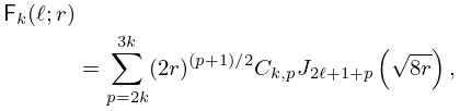
the factor

(r/4)^{-1/6}

in Carlson (1995, (2.18)) is changed to

(r/5)^{-1/8}

when the following polynomial of degree 7 (the same for both) is used instead of its first seven terms: … ►Accurate values of

F\left(\phi,k\right)-E\left(\phi,k\right)

for

k^{2}

near 0 can be obtained from

R_{D}

by (19.2.6) and (19.25.13). … ►

F\left(\phi,k\right)

can be evaluated by using (19.25.5). …A summary for

F\left(\phi,k\right)

is given in Gautschi (1975, §3). …

18: 12.14 The Function $W\left(a,x\right)$

… ►For the modulus functions

\widetilde{F}(a,x)

and

\widetilde{G}(a,x)

see §12.14(x). … ►the branch of

\operatorname{ph}

being zero when

a=0

and defined by continuity elsewhere. … ►Other expansions, involving

\cos\left(\tfrac{1}{4}x^{2}\right)

and

\sin\left(\tfrac{1}{4}x^{2}\right)

, can be obtained from (12.4.3) to (12.4.6) by replacing

a

-ia

and

z

xe^{\ifrac{\pi i}{4}}

; see Miller (1955, p. 80), and also (12.14.15) and (12.14.16). … ►where

k

is defined in (12.14.5), and

\widetilde{F}(a,x)

(

>

0),

\widetilde{\theta}(a,x)

\widetilde{G}(a,x)

(

>

0), and

\widetilde{\psi}(a,x)

are real.

\widetilde{F}

\widetilde{G}

is the modulus and

\widetilde{\theta}

\widetilde{\psi}

is the corresponding phase. …

19: 19.5 Maclaurin and Related Expansions

… ►where

{{}_{2}F_{1}}

is the Gauss hypergeometric function (§§15.1 and 15.2(i)). …where

{F_{1}}\left(\alpha;\beta,\beta^{\prime};\gamma;x,y\right)

is an Appell function (§16.13). … ►

19.5.5

q=\exp\left(-\pi{K^{\prime}}\left(k\right)/K\left(k\right)\right)=r+8r^{2}+84r% ^{3}+992r^{4}+\cdots,

r=\frac{1}{16}k^{2}

0\leq k\leq 1

ⓘ

Symbols:: $\pi$ : the ratio of the circumference of a circle to its diameter, ${K^{\prime}}\left(\NVar{k}\right)$ : Legendre’s complementary complete elliptic integral of the first kind, $K\left(\NVar{k}\right)$ : Legendre’s complete elliptic integral of the first kind, $\exp\NVar{z}$ : exponential function, $q$ : nome and $k$ : real or complex modulus
Referenced by:: §19.5
Permalink:: http://dlmf.nist.gov/19.5.E5
Encodings:: pMML, png, TeX
See also:: Annotations for §19.5 and Ch.19

… ►Series expansions of

F\left(\phi,k\right)

and

E\left(\phi,k\right)

are surveyed and improved in Van de Vel (1969), and the case of

F\left(\phi,k\right)

is summarized in Gautschi (1975, §1.3.2). For series expansions of

\Pi\left(\phi,\alpha^{2},k\right)

when

|\alpha^{2}|<1

see Erdélyi et al. (1953b, §13.6(9)). …

20: 33.12 Asymptotic Expansions for Large $\eta$

… ►

33.12.3

{F_{0}'\left(\eta,\rho\right)\atop G_{0}'\left(\eta,\rho\right)}\sim-\pi^{1/2}% (2\eta)^{-1/6}\left\{{\operatorname{Ai}\left(x\right)\atop\operatorname{Bi}% \left(x\right)}\left(\frac{B_{1}^{\prime}+xA_{1}}{\mu}+\frac{B_{2}^{\prime}+xA% _{2}}{\mu^{2}}+\cdots\right)+{\operatorname{Ai}'\left(x\right)\atop% \operatorname{Bi}'\left(x\right)}\left(\frac{B_{1}+A_{1}^{\prime}}{\mu}+\frac{% B_{2}+A_{2}^{\prime}}{\mu^{2}}+\cdots\right)\right\},

ⓘ

Symbols:: $\operatorname{Ai}\left(\NVar{z}\right)$ : Airy function, $\operatorname{Bi}\left(\NVar{z}\right)$ : Airy function, $\sim$ : Poincaré asymptotic expansion, $\pi$ : the ratio of the circumference of a circle to its diameter, $G_{\NVar{\ell}}\left(\NVar{\eta},\NVar{\rho}\right)$ : irregular Coulomb radial function, $F_{\NVar{\ell}}\left(\NVar{\eta},\NVar{\rho}\right)$ : regular Coulomb radial function, $\rho$ : nonnegative real variable, $\eta$ : real parameter, $x$ : variable, $\mu$ : variable, $A_{j}$ : coefficients and $B_{j}$ : coefficients
A&S Ref:: 14.4.10
Permalink:: http://dlmf.nist.gov/33.12.E3
Encodings:: pMML, png, TeX
See also:: Annotations for §33.12(i), §33.12 and Ch.33

… ►

33.12.6

{F_{0}\left(\eta,2\eta\right)\atop{3^{-\ifrac{1}{2}}G_{0}\left(\eta,2\eta% \right)}}\sim\frac{\Gamma\left(\frac{1}{3}\right)\omega^{1/2}}{2\sqrt{\pi}}% \left(1\mp\frac{2}{35}\frac{\Gamma\left(\frac{2}{3}\right)}{\Gamma\left(\frac{% 1}{3}\right)}\frac{1}{\omega^{4}}-\frac{8}{2025}\frac{1}{\omega^{6}}\mp\frac{5% 792}{46\,06875}\frac{\Gamma\left(\frac{2}{3}\right)}{\Gamma\left(\frac{1}{3}% \right)}\frac{1}{\omega^{10}}-\cdots\right),

ⓘ

Symbols:: $\Gamma\left(\NVar{z}\right)$ : gamma function, $\sim$ : Poincaré asymptotic expansion, $\pi$ : the ratio of the circumference of a circle to its diameter, $G_{\NVar{\ell}}\left(\NVar{\eta},\NVar{\rho}\right)$ : irregular Coulomb radial function, $F_{\NVar{\ell}}\left(\NVar{\eta},\NVar{\rho}\right)$ : regular Coulomb radial function, $\eta$ : real parameter and $\omega$ : factor
Permalink:: http://dlmf.nist.gov/33.12.E6
Encodings:: pMML, png, TeX
See also:: Annotations for §33.12(i), §33.12 and Ch.33

►

33.12.7

{F_{0}'\left(\eta,2\eta\right)\atop{3^{-\ifrac{1}{2}}G_{0}'\left(\eta,2\eta% \right)}}\sim\frac{\Gamma\left(\frac{2}{3}\right)}{2\sqrt{\pi}\omega^{1/2}}% \left(\pm 1+\frac{1}{15}\frac{\Gamma\left(\frac{1}{3}\right)}{\Gamma\left(% \frac{2}{3}\right)}\frac{1}{\omega^{2}}\pm\frac{2}{14175}\frac{1}{\omega^{6}}+% \frac{1436}{23\,38875}\frac{\Gamma\left(\frac{1}{3}\right)}{\Gamma\left(\frac{% 2}{3}\right)}\frac{1}{\omega^{8}}\pm\cdots\right),

ⓘ

Symbols:: $\Gamma\left(\NVar{z}\right)$ : gamma function, $\sim$ : Poincaré asymptotic expansion, $\pi$ : the ratio of the circumference of a circle to its diameter, $G_{\NVar{\ell}}\left(\NVar{\eta},\NVar{\rho}\right)$ : irregular Coulomb radial function, $F_{\NVar{\ell}}\left(\NVar{\eta},\NVar{\rho}\right)$ : regular Coulomb radial function, $\eta$ : real parameter and $\omega$ : factor
Referenced by:: §33.12(i)
Permalink:: http://dlmf.nist.gov/33.12.E7
Encodings:: pMML, png, TeX
See also:: Annotations for §33.12(i), §33.12 and Ch.33

… ►For asymptotic expansions of

F_{\ell}\left(\eta,\rho\right)

and

G_{\ell}\left(\eta,\rho\right)

when

\eta\to\pm\infty

see Temme (2015, Chapter 31). … ►Then, by application of the results given in §§2.8(iii) and 2.8(iv), two sets of asymptotic expansions can be constructed for

F_{\ell}\left(\eta,\rho\right)

and

G_{\ell}\left(\eta,\rho\right)

when

\eta\to\infty

. …

11—20 of 769 matching pages

11: 18.5 Explicit Representations

12: 27.2 Functions

13: 33.20 Expansions for Small | ϵ |

14: 16.4 Argument Unity

15: 19.24 Inequalities

16: 26.13 Permutations: Cycle Notation

17: 19.36 Methods of Computation

18: 12.14 The Function W ⁡ ( a , x )

19: 19.5 Maclaurin and Related Expansions

20: 33.12 Asymptotic Expansions for Large η

13: 33.20 Expansions for Small $|\epsilon|$

18: 12.14 The Function $W\left(a,x\right)$

20: 33.12 Asymptotic Expansions for Large $\eta$