how to order clomid no prescription online cheaP-pHarma.com/?id=1738

SearchAdvancedHelp

(0.037 seconds)

11—20 of 873 matching pages

11: 13.5 Continued Fractions

… ►This continued fraction converges to the meromorphic function of $z$ on the left-hand side everywhere in $ℂ$. For more details on how a continued fraction converges to a meromorphic function see Jones and Thron (1980). … ►This continued fraction converges to the meromorphic function of $z$ on the left-hand side throughout the sector . …

12: 13.17 Continued Fractions

… ►This continued fraction converges to the meromorphic function of $z$ on the left-hand side for all $z\in ℂ$. For more details on how a continued fraction converges to a meromorphic function see Jones and Thron (1980). … ►This continued fraction converges to the meromorphic function of $z$ on the left-hand side throughout the sector . …

13: 18.40 Methods of Computation

… ►

A numerical approach to the recursion coefficients and quadrature abscissas and weights

… ►See Gautschi (1983) for examples of numerically stable and unstable use of the above recursion relations, and how one can then usefully differentiate between numerical results of low and high precision, as produced thereby. ►Having now directly connected computation of the quadrature abscissas and weights to the moments, what follows uses these for a Stieltjes–Perron inversion to regain $w(x)$. … ►The question is then: how is this possible given only $F_N(z)$, rather than $F(z)$ itself? $F_N(z)$ often converges to smooth results for $z$ off the real axis for $\mathrm{\Im }z$ at a distance greater than the pole spacing of the $x_n$, this may then be followed by approximate numerical analytic continuation via fitting to lower order continued fractions (either Padé, see §3.11(iv), or pointwise continued fraction approximants, see Schlessinger (1968, Appendix)), to $F_N(z)$ and evaluating these on the real axis in regions of higher pole density that those of the approximating function. Results of low ($2$ to $3$ decimal digits) precision for $w(x)$ are easily obtained for $N\sim 10$ to $20$. …

14: 33.21 Asymptotic Approximations for Large $|r|$

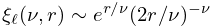
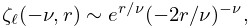
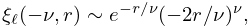
… ►We indicate here how to obtain the limiting forms of $f(ϵ,\mathrm{\ell };r)$, $h(ϵ,\mathrm{\ell };r)$, $s(ϵ,\mathrm{\ell };r)$, and $c(ϵ,\mathrm{\ell };r)$ as $r\to \pm \mathrm{\infty }$, with $ϵ$ and $\mathrm{\ell }$ fixed, in the following cases: ►

When $r\to \pm \mathrm{\infty }$ with $ϵ>0$, Equations (33.16.4)–(33.16.7) are combined with (33.10.1).

►

When $r\to \pm \mathrm{\infty }$ with , Equations (33.16.10)–(33.16.13) are combined with

33.21.1

${\zeta }_{\mathrm{\ell }}(\nu ,r)\sim {\mathrm{e}}^{-r/\nu }{(2r/\nu )}^{\nu },$

${\xi }_{\mathrm{\ell }}(\nu ,r)\sim {\mathrm{e}}^{r/\nu }{(2r/\nu )}^{-\nu }$ , $r\to \mathrm{\infty }$,

ⓘ

Symbols:

$\sim$: asymptotic equality, $\mathrm{e}$: base of natural logarithm, $\mathrm{\ell }$: nonnegative integer, $r$: real variable, $\nu$: parameter, ${\zeta }_{\mathrm{\ell }}(\nu ,r)$: function and ${\xi }_{\mathrm{\ell }}(\nu ,r)$: function

Permalink:

http://dlmf.nist.gov/33.21.E1

Encodings:

pMML, pMML, png, png, TeX, TeX

See also:

Annotations for §33.21(i), §33.21 and Ch.33

33.21.2

${\zeta }_{\mathrm{\ell }}(-\nu ,r)\sim {\mathrm{e}}^{r/\nu }{(-2r/\nu )}^{-\nu },$

${\xi }_{\mathrm{\ell }}(-\nu ,r)\sim {\mathrm{e}}^{-r/\nu }{(-2r/\nu )}^{\nu },$ $r\to -\mathrm{\infty }$.

ⓘ

Symbols:

$\sim$: asymptotic equality, $\mathrm{e}$: base of natural logarithm, $\mathrm{\ell }$: nonnegative integer, $r$: real variable, $\nu$: parameter, ${\zeta }_{\mathrm{\ell }}(\nu ,r)$: function and ${\xi }_{\mathrm{\ell }}(\nu ,r)$: function

Permalink:

http://dlmf.nist.gov/33.21.E2

Encodings:

pMML, pMML, png, png, TeX, TeX

See also:

Annotations for §33.21(i), §33.21 and Ch.33

Corresponding approximations for $s(ϵ,\mathrm{\ell };r)$ and $c(ϵ,\mathrm{\ell };r)$ as $r\to \mathrm{\infty }$ can be obtained via (33.16.17), and as $r\to -\mathrm{\infty }$ via (33.16.18).

►

When $r\to \pm \mathrm{\infty }$ with $ϵ=0$, combine (33.20.1), (33.20.2) with §§10.7(ii), 10.30(ii).

… ►For asymptotic expansions of $f(ϵ,\mathrm{\ell };r)$ and $h(ϵ,\mathrm{\ell };r)$ as $r\to \pm \mathrm{\infty }$ with $ϵ$ and $\mathrm{\ell }$ fixed, see Curtis (1964a, §6).

15: 5.4 Special Values and Extrema

… ►

5.4.7 $$\mathrm{\Gamma }\left(\frac{1}{3}\right)=\mathrm{2.67893\hspace{0.33em}85347\hspace{0.33em}07747\hspace{0.33em}63365}\mathrm{\dots },$$

ⓘ

Symbols:

$\mathrm{\Gamma }\left(z\right)$: gamma function

A&S Ref:

6.1.11 (where the value is computed to 10D.)

Notes:

For more digits see OEIS Sequence A073005; see also Sloane (2003).

Permalink:

http://dlmf.nist.gov/5.4.E7

Encodings:

pMML, png, TeX

See also:

Annotations for §5.4(i), §5.4 and Ch.5

►

5.4.8 $$\mathrm{\Gamma }\left(\frac{2}{3}\right)=\mathrm{1.35411\hspace{0.33em}79394\hspace{0.33em}26400\hspace{0.33em}41694}\mathrm{\dots },$$

ⓘ

Symbols:

$\mathrm{\Gamma }\left(z\right)$: gamma function

A&S Ref:

6.1.13 (where the value is computed to 10D.)

Notes:

For more digits see OEIS Sequence A073006; see also Sloane (2003).

Permalink:

http://dlmf.nist.gov/5.4.E8

Encodings:

pMML, png, TeX

See also:

Annotations for §5.4(i), §5.4 and Ch.5

►

5.4.9 $$\mathrm{\Gamma }\left(\frac{1}{4}\right)=\mathrm{3.62560\hspace{0.33em}99082\hspace{0.33em}21908\hspace{0.33em}31193}\mathrm{\dots },$$

ⓘ

Symbols:

$\mathrm{\Gamma }\left(z\right)$: gamma function

A&S Ref:

6.1.10 (where the value is computed to 10D.)

Notes:

For more digits see OEIS Sequence A068466; see also Sloane (2003).

Permalink:

http://dlmf.nist.gov/5.4.E9

Encodings:

pMML, png, TeX

See also:

Annotations for §5.4(i), §5.4 and Ch.5

… ►As $n\to \mathrm{\infty }$, ►

5.4.20 $$x_n=-n+\frac{1}{\pi }\arctan \left(\frac{\pi }{\ln n}\right)+O\left(\frac{1}{n{(\ln n)}^2}\right).$$

ⓘ

Symbols:

$O\left(x\right)$: order not exceeding, $\pi$: the ratio of the circumference of a circle to its diameter, $\arctan z$: arctangent function, $\ln z$: principal branch of logarithm function, $n$: nonnegative integer and $x$: real variable

A&S Ref:

6.3.20 (The error estimate has been improved.)

Referenced by:

§5.4(iii)

Permalink:

http://dlmf.nist.gov/5.4.E20

Encodings:

pMML, png, TeX

See also:

Annotations for §5.4(iii), §5.4 and Ch.5

…

16: Bibliography G

… ►

Stable computation of high order Gauss quadrature rules using discretization for measures in radiation transfer. J. Quant. Spectrosc. Radiat. Transfer 68 (2), pp. 213–223.

ⓘ

Referenced by:

§18.39(iii).

Encodings:

BibTeX

… ►

How and how not to check Gaussian quadrature formulae. BIT 23 (2), pp. 209–216.

ⓘ

External Links:

ISSN 0006-3835, Document, MathReview (G. A. Evans), ZentralBlatt

Referenced by:

§18.40(ii), §3.5(v), §9.17(iii).

Encodings:

BibTeX

… ►

Evaluation of the modified Bessel function of the third kind of imaginary orders. J. Comput. Phys. 175 (2), pp. 398–411.

ⓘ

External Links:

ISSN 0021-9991, Document, MathReview (J. P. Singhal), ZentralBlatt

Referenced by:

§10.74(viii).

Encodings:

BibTeX

… ►

Algorithm 831: Modified Bessel functions of imaginary order and positive argument. ACM Trans. Math. Software 30 (2), pp. 159–164.

ⓘ

External Links:

ISSN 0098-3500, Document, GAMS (module 831; package TOMS), MathReview Entry, ZentralBlatt

Referenced by:

1st item.

Encodings:

BibTeX

►

Computing solutions of the modified Bessel differential equation for imaginary orders and positive arguments. ACM Trans. Math. Software 30 (2), pp. 145–158.

ⓘ

External Links:

ISSN 0098-3500, Document, MathReview, ZentralBlatt

Referenced by:

§10.74(viii).

Encodings:

BibTeX

…

17: 3.6 Linear Difference Equations

… ►In practice, however, problems of severe instability often arise and in §§3.6(ii)–3.6(vii) we show how these difficulties may be overcome. … ►Suppose again that $f_0\ne 0$, $w_0$ is given, and we wish to calculate $w_1,w_2,\mathrm{\dots },w_M$ to a prescribed relative accuracy $ϵ$ for a given value of $M$. … ►

§3.6(vii) Linear Difference Equations of Other Orders

►Similar considerations apply to the first-order equation …Thus in the inhomogeneous case it may sometimes be necessary to recur backwards to achieve stability. …

18: 1.13 Differential Equations

… ►(More generally in (1.13.5) for $n$th-order differential equations, $f(z)$ is the coefficient multiplying the $(n-1)$th-order derivative of the solution divided by the coefficient multiplying the $n$th-order derivative of the solution, see Ince (1926, §5.2).) … ►For extensions of these results to linear homogeneous differential equations of arbitrary order see Spigler (1984). … ►For an extensive collection of solutions of differential equations of the first, second, and higher orders see Kamke (1977). … ►The functions $u(x)$ which correspond to these being eigenfunctions. … ►

Transformation to Liouville normal Form

…

19: 3.2 Linear Algebra

… ►To solve the system … ►During this reduction process we store the multipliers ${\mathrm{\ell }}_{jk}$ that are used in each column to eliminate other elements in that column. … ►

§3.2(iii) Condition of Linear Systems

… ►where $𝐱$ and $𝐲$ are the normalized right and left eigenvectors of $𝐀$ corresponding to the eigenvalue $\lambda$. … ►Lanczos’ method is related to Gauss quadrature considered in §3.5(v). …

20: 19.36 Methods of Computation

… ►In the Appendix of the last reference it is shown how to compute $R_J$ without computing $R_C$ more than once. … ►As $n\to \mathrm{\infty }$, $c_n$, $a_n$, and $t_n$ converge quadratically to limits $0$, $M$, and $T$, respectively; hence … ►To (19.36.6) add … ►(19.22.20) reduces to $0=0$ if $p=x$ or $p=y$, and (19.22.19) reduces to $0=0$ if $z=x$ or $z=y$. … ►Quadratic transformations can be applied to compute Bulirsch’s integrals (§19.2(iii)). …