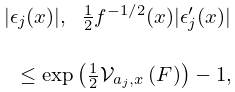
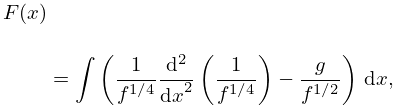
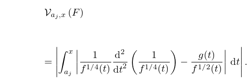
error control

SearchAdvancedHelp

(0.002 seconds)

5 matching pages

1: 2.7 Differential Equations

… ►

2.7.23 $$|{ϵ}_j(x)|,\frac{1}{2}{f}^{-1/2}(x)|{ϵ}_j^{\prime }(x)|\le \exp \left(\frac{1}{2}{𝒱}_{a_j,x}\left(F\right)\right)-1,$$ $j=1,2$,

ⓘ

Symbols:

$\exp z$: exponential function, ${𝒱}_{a,b}\left(f\right)$: total variation, $(a_1,a_2)$: interval, ${ϵ}_j(x)$: function and $F$: error-control function

Permalink:

http://dlmf.nist.gov/2.7.E23

Encodings:

pMML, png, TeX

See also:

Annotations for §2.7(iii), §2.7(iii), §2.7 and Ch.2

… ►Here $F(x)$ is the error-control function ►

2.7.24 $$F(x)=\int \left(\frac{1}{f^{1/4}}\frac{d^2}{{dx}^2}\left(\frac{1}{f^{1/4}}\right)-\frac{g}{f^{1/2}}\right)dx,$$

ⓘ

Symbols:

$\frac{df}{dx}$: derivative of $f$ with respect to $x$ , $dx$: differential of $x$ , $\int$: integral and $F$: error-control function

Permalink:

http://dlmf.nist.gov/2.7.E24

Encodings:

pMML, png, TeX

See also:

Annotations for §2.7(iii), §2.7(iii), §2.7 and Ch.2

… ►

2.7.25 $${𝒱}_{a_j,x}\left(F\right)=\left|{\int }_{a_j}^x\left|\frac{1}{f^{1/4}(t)}\frac{d^2}{{dt}^2}\left(\frac{1}{f^{1/4}(t)}\right)-\frac{g(t)}{f^{1/2}(t)}\right|dt\right|.$$

ⓘ

Symbols:

$\frac{df}{dx}$: derivative of $f$ with respect to $x$ , $dx$: differential of $x$ , $\int$: integral, ${𝒱}_{a,b}\left(f\right)$: total variation, $(a_1,a_2)$: interval and $F$: error-control function

Referenced by:

Erratum (V1.1.2) for Equation (2.7.25)

Permalink:

http://dlmf.nist.gov/2.7.E25

Encodings:

pMML, png, TeX

Correction (effective with 1.1.2):

The integrand was corrected so that the absolute value does not include the differential. Also an absolute value was introduced on the right-hand side to ensure a non-negative value.

See also:

Annotations for §2.7(iii), §2.7(iii), §2.7 and Ch.2

…

2: Bibliography K

… ►

Algorithm 421. Complex gamma function with error control. Comm. ACM 15 (4), pp. 271–272.

ⓘ

External Links:

ISSN 0001-0782, Document

Referenced by:

§5.24(iv).

Encodings:

BibTeX

…

3: 15.19 Methods of Computation

… ►The accuracy is controlled and validated by a running error analysis coupled with interval arithmetic.

4: 13.29 Methods of Computation

… ►The accuracy is controlled and validated by a running error analysis coupled with interval arithmetic.

5: 19.38 Approximations

… ►Minimax polynomial approximations (§3.11(i)) for $K\left(k\right)$ and $E\left(k\right)$ in terms of $m=k^2$ with can be found in Abramowitz and Stegun (1964, §17.3) with maximum absolute errors ranging from 4×10⁻⁵ to 2×10⁻⁸. Approximations of the same type for $K\left(k\right)$ and $E\left(k\right)$ for are given in Cody (1965a) with maximum absolute errors ranging from 4×10⁻⁵ to 4×10⁻¹⁸. … ►The accuracy is controlled by the number of terms retained in the approximation; for real variables the number of significant figures appears to be roughly twice the number of terms retained, perhaps even for $\varphi$ near $\pi /2$ with the improvements made in the 1970 reference. …