value%20at%20T%3D0

SearchAdvancedHelp

(0.004 seconds)

11—20 of 784 matching pages

11: 24.20 Tables

… ►Abramowitz and Stegun (1964, Chapter 23) includes exact values of ${\sum }_{k=1}^m{k}^n$, $m=1(1)100$, $n=1(1)10$; ${\sum }_{k=1}^{\mathrm{\infty }}{k}^{-n}$, ${\sum }_{k=1}^{\mathrm{\infty }}{(-1)}^{k-1}{k}^{-n}$, ${\sum }_{k=0}^{\mathrm{\infty }}{(2k+1)}^{-n}$, $n=1,2,\mathrm{\dots }$, 20D; ${\sum }_{k=0}^{\mathrm{\infty }}{(-1)}^k{(2k+1)}^{-n}$, $n=1,2,\mathrm{\dots }$, 18D. ►Wagstaff (1978) gives complete prime factorizations of $N_n$ and $E_n$ for $n=20(2)60$ and $n=8(2)42$, respectively. …

12: Wolter Groenevelt

… ► 1976 in Leidschendam, the Netherlands) is an Associate Professor at the Delft University of Technology in Delft, The Netherlands. … ► in mathematics at the Delft University of Technology in 2004. … ►As of September 20, 2022, Groenevelt performed a complete analysis and acted as main consultant for the update of the source citation and proof metadata for every formula in Chapter 18 Orthogonal Polynomials. …

13: 22.3 Graphics

… ►Line graphs of the functions $\mathrm{sn}(x,k)$, $\mathrm{cn}(x,k)$, $\mathrm{dn}(x,k)$, $\mathrm{cd}(x,k)$, $\mathrm{sd}(x,k)$, $\mathrm{nd}(x,k)$, $\mathrm{dc}(x,k)$, $\mathrm{nc}(x,k)$, $\mathrm{sc}(x,k)$, $\mathrm{ns}(x,k)$, $\mathrm{ds}(x,k)$, and $\mathrm{cs}(x,k)$ for representative values of real $x$ and real $k$ illustrating the near trigonometric ($k=0$), and near hyperbolic ($k=1$) limits. … ►

►

►

Figure 22.3.13: $\mathrm{sn}(x,k)$ for $k=1-{\mathrm{e}}^{-n}$, $n=0$ to 20, $-5\pi \le x\le 5\pi$. Magnify 3D Help

… ►In the graphics shown in this subsection height corresponds to the absolute value of the function and color to the phase. … ►In Figures 22.3.24 and 22.3.25, height corresponds to the absolute value of the function and color to the phase. … ►

►►

Figure 22.3.28: Density plot of $|\mathrm{sn}(20,k)|$ as a function of complex $k^2$, $-10\le \mathrm{\Re }\left(k^2\right)\le 20$, $-10\le \mathrm{\Im }\left(k^2\right)\le 10$. … Magnify

…

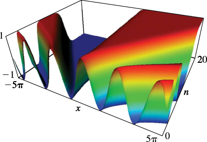
14: 3.4 Differentiation

… ►For the values of $n_0$ and $n_1$ used in the formulas below …where $c_n$ is defined by (3.3.12), with numerical values as in §3.3(ii). … ►Taking $C$ to be a circle of radius $r$ centered at $x_0$, we obtain … ►With the choice $r=k$ (which is crucial when $k$ is large because of numerical cancellation) the integrand equals ${\mathrm{e}}^k$ at the dominant points $\theta =0,2\pi$, and in combination with the factor $k^{-k}$ in front of the integral sign this gives a rough approximation to $1/k!$. … ►For additional formulas involving values of ${\nabla }^{2}u$ and ${\nabla }^{4}u$ on square, triangular, and cubic grids, see Collatz (1960, Table VI, pp. 542–546). …

15: 28.35 Tables

§28.35 Tables

… ►

Ince (1932) includes eigenvalues $a_n$, $b_n$, and Fourier coefficients for $n=0$ or $1(1)6$, $q=0(1)10(2)20(4)40$; 7D. Also ${\mathrm{ce}}_n(x,q)$, ${\mathrm{se}}_n(x,q)$ for $q=0(1)10$, $x=1(1)90$, corresponding to the eigenvalues in the tables; 5D. Notation: $a_n={\mathrm{𝑏𝑒}}_n-2q$, $b_n={\mathrm{𝑏𝑜}}_n-2q$.

►

Kirkpatrick (1960) contains tables of the modified functions ${\mathrm{Ce}}_n(x,q)$, ${\mathrm{Se}}_{n+1}(x,q)$ for $n=0(1)5$, $q=1(1)20$, $x=0.1(.1)1$; 4D or 5D.

►

National Bureau of Standards (1967) includes the eigenvalues $a_n\left(q\right)$, $b_n\left(q\right)$ for $n=0(1)3$ with $q=0(.2)20(.5)37(1)100$, and $n=4(1)15$ with $q=0(2)100$; Fourier coefficients for ${\mathrm{ce}}_n(x,q)$ and ${\mathrm{se}}_n(x,q)$ for $n=0(1)15$, $n=1(1)15$, respectively, and various values of $q$ in the interval $[0,100]$; joining factors $g_{e,n}(\sqrt{q})$, $f_{e,n}(\sqrt{q})$ for $n=0(1)15$ with $q=0(.5\text{ to }10)100$ (but in a different notation). Also, eigenvalues for large values of $q$. Precision is generally 8D.

… ►

Zhang and Jin (1996, pp. 521–532) includes the eigenvalues $a_n\left(q\right)$, $b_{n+1}\left(q\right)$ for $n=0(1)4$, $q=0(1)50$; $n=0(1)20$ ($a$’s) or 19 ($b$’s), $q=1,3,5,10,15,25,50(50)200$. Fourier coefficients for ${\mathrm{ce}}_n(x,10)$, ${\mathrm{se}}_{n+1}(x,10)$, $n=0(1)7$. Mathieu functions ${\mathrm{ce}}_n(x,10)$, ${\mathrm{se}}_{n+1}(x,10)$, and their first $x$-derivatives for $n=0(1)4$, $x=0(5^{\circ }){90}^{\circ }$. Modified Mathieu functions ${\mathrm{Mc}}_n^{(j)}(x,\sqrt{10})$, ${\mathrm{Ms}}_{n+1}^{(j)}(x,\sqrt{10})$, and their first $x$-derivatives for $n=0(1)4$, $j=1,2$, $x=0(.2)4$. Precision is mostly 9S.

…

16: 10.3 Graphics

… ►In the graphics shown in this subsection, height corresponds to the absolute value of the function and color to the phase. … ►

►

►

Figure 10.3.10: $H_0^{(1)}\left(x+\mathrm{i}y\right)$, $-10\le x\le 5$, $-2.8\le y\le 4$. Principal value. … Magnify 3D Help

… ►

►

►

Figure 10.3.12: $H_1^{(1)}\left(x+\mathrm{i}y\right)$, $-10\le x\le 5$, $-2.8\le y\le 4$. Principal value. … Magnify 3D Help

… ►

►

►

Figure 10.3.14: $H_5^{(1)}\left(x+\mathrm{i}y\right)$, $-20\le x\le 10$, $-4\le y\le 4$. Principal value. … Magnify 3D Help

►

►

►

Figure 10.3.15: $J_{5.5}\left(x+\mathrm{i}y\right)$, $-10\le x\le 10$, $-4\le y\le 4$. Principal value. … Magnify 3D Help

…

17: Bibliography B

… ►

Pionic atoms. Annual Review of Nuclear and Particle Science 20, pp. 467–508.

ⓘ

External Links:

Document

Referenced by:

§33.22(iv).

Encodings:

BibTeX

… ►

A program for computing the Riemann zeta function for complex argument. Comput. Phys. Comm. 20 (3), pp. 441–445.

ⓘ

Notes:

Double-precision Fortran, maximum accuracy 10S.

External Links:

Document, Code, ZentralBlatt

Referenced by:

1st item.

Encodings:

BibTeX

… ►

Coulomb functions (negative energies). Comput. Phys. Comm. 20 (3), pp. 447–458.

ⓘ

Notes:

Double-precision Fortran code.

External Links:

Document, Code

Referenced by:

1st item, 4th item.

Encodings:

BibTeX

… ►

Some solutions of the problem of forced convection. Philos. Mag. Series 7 20, pp. 322–343.

ⓘ

External Links:

Document, ZentralBlatt

Referenced by:

§10.73(iv).

Encodings:

BibTeX

… ►

Bessel functions and modular relations of higher type and hyperbolic differential equations. Comm. Sém. Math. Univ. Lund [Medd. Lunds Univ. Mat. Sem.] 1952 (Tome Supplementaire), pp. 12–20.

ⓘ

External Links:

MathReview (S. C. van Veen), ZentralBlatt

Referenced by:

§35.5(i).

Encodings:

BibTeX

…

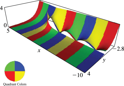
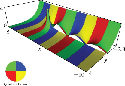
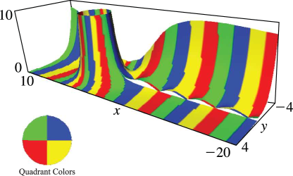
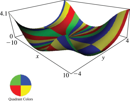
18: 36.5 Stokes Sets

… ►In the following subsections, only Stokes sets involving at least one real saddle are included unless stated otherwise. … ►The Stokes set consists of the rays $\mathrm{ph}x=\pm 2\pi /3$ in the complex $x$-plane. … ►

$K=3$. Swallowtail

… ►This consists of three separate cusp-edged sheets connected to the cusp-edged sheets of the bifurcation set, and related by rotation about the $z$-axis by $2\pi /3$. … ►such that $u>\frac{1}{3}$. …

19: 7.24 Approximations

… ►

Cody (1969) provides minimax rational approximations for $\mathrm{erf}x$ and $\mathrm{erfc}x$. The maximum relative precision is about 20S.

… ►

Cody et al. (1970) gives minimax rational approximations to Dawson’s integral $F\left(x\right)$ (maximum relative precision 20S–22S).

… ►

Luke (1969b, pp. 323–324) covers $\frac{1}{2}\sqrt{\pi }\mathrm{erf}x$ and ${\mathrm{e}}^{x^2}F\left(x\right)$ for $-3\le x\le 3$ (the Chebyshev coefficients are given to 20D); $\sqrt{\pi }x{\mathrm{e}}^{x^2}\mathrm{erfc}x$ and $2xF\left(x\right)$ for $x\ge 3$ (the Chebyshev coefficients are given to 20D and 15D, respectively). Coefficients for the Fresnel integrals are given on pp. 328–330 (20D).

►

Bulirsch (1967) provides Chebyshev coefficients for the auxiliary functions $\mathrm{f}\left(x\right)$ and $\mathrm{g}\left(x\right)$ for $x\ge 3$ (15D).

… ►

Luke (1969b, vol. 2, pp. 422–435) gives main diagonal Padé approximations for $F\left(z\right)$, $\mathrm{erf}z$, $\mathrm{erfc}z$, $C\left(z\right)$, and $S\left(z\right)$; approximate errors are given for a selection of $z$-values.

20: Gergő Nemes

… ► 1988 in Szeged, Hungary) is a Research Fellow at the Alfréd Rényi Institute of Mathematics in Budapest, Hungary. … ►As of September 20, 2021, Nemes performed a complete analysis and acted as main consultant for the update of the source citation and proof metadata for every formula in Chapter 25 Zeta and Related Functions. …