sum rules

SearchAdvancedHelp

(0.001 seconds)

11—19 of 19 matching pages

11: 1.11 Zeros of Polynomials

… ►

Descartes’ Rule of Signs

… ►

… ►The sum and product of the roots are respectively $-b/a$ and $c/a$. …

12: 13.29 Methods of Computation

… ►In Allasia and Besenghi (1991) and Allasia and Besenghi (1987a) the high accuracy of the trapezoidal rule for the computation of Kummer functions is described. … ►

13.29.3 $${\mathrm{e}}^{-\frac{1}{2}z}=\sum _{s=0}^{\mathrm{\infty }}\frac{{\left(2\mu \right)}_s{\left(\frac{1}{2}+\mu -\kappa \right)}_s}{{\left(2\mu \right)}_{2s}s!}{(-z)}^{s}y(s),$$

ⓘ

Symbols:

${\left(a\right)}_n$: Pochhammer’s symbol (or shifted factorial), $\mathrm{e}$: base of natural logarithm, $!$: factorial (as in $n!$), $s$: nonnegative integer, $z$: complex variable and $y(n)$: solution

Permalink:

http://dlmf.nist.gov/13.29.E3

Encodings:

pMML, png, TeX

See also:

Annotations for §13.29(iv), §13.29(iv), §13.29 and Ch.13

… ►

13.29.7 $$z^{-a}=\sum _{s=0}^{\mathrm{\infty }}\frac{{\left(a-b+1\right)}_s}{s!}w(s),$$

ⓘ

Symbols:

${\left(a\right)}_n$: Pochhammer’s symbol (or shifted factorial), $!$: factorial (as in $n!$), $s$: nonnegative integer and $z$: complex variable

Permalink:

http://dlmf.nist.gov/13.29.E7

Encodings:

pMML, png, TeX

See also:

Annotations for §13.29(iv), §13.29(iv), §13.29 and Ch.13

…

13: 18.40 Methods of Computation

… ►

Derivative Rule Approach

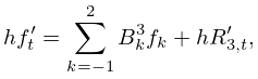
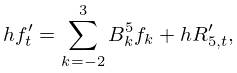
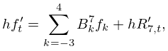
►An alternate, and highly efficient, approach follows from the derivative rule conjecture, see Yamani and Reinhardt (1975), and references therein, namely that … ►

►►

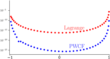
Figure 18.40.2: Derivative Rule inversions for $w^{\mathrm{RCP}}(x)$ carried out via Lagrange and PWCF interpolations. …For the derivative rule Lagrange interpolation (red points) gives $\sim 15$ digits in the central region, while PWCF interpolation (blue points) gives $\sim 25$. Magnify

►Further, exponential convergence in $N$, via the Derivative Rule, rather than the power-law convergence of the histogram methods, is found for the inversion of Gegenbauer, Attractive, as well as Repulsive, Coulomb–Pollaczek, and Hermite weights and zeros to approximate $w(x)$ for these OP systems on $x\in [-1,1]$ and $(-\mathrm{\infty },\mathrm{\infty })$ respectively, Reinhardt (2018), and Reinhardt (2021b), Reinhardt (2021a). …

14: 3.10 Continued Fractions

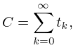
… ►can be converted into a continued fraction $C$ of type (3.10.1), and with the property that the $n$th convergent $C_n=A_n/B_n$ to $C$ is equal to the $n$th partial sum of the series in (3.10.3), that is, … ►We continue by means of the rhombus rule … ►

3.10.14 $$C=\sum _{k=0}^{\mathrm{\infty }}{t}_k,$$

ⓘ

Symbols:

$C$: continued fraction

Permalink:

http://dlmf.nist.gov/3.10.E14

Encodings:

pMML, png, TeX

See also:

Annotations for §3.10(iii), §3.10(iii), §3.10 and Ch.3

… ►The $n$th partial sum $t_0+t_1+\mathrm{\cdots }+t_{n-1}$ equals the $n$th convergent of (3.10.13), $n=1,2,3,\mathrm{\dots }$. …

15: Bibliography G

… ►

Stable computation of high order Gauss quadrature rules using discretization for measures in radiation transfer. J. Quant. Spectrosc. Radiat. Transfer 68 (2), pp. 213–223.

ⓘ

Referenced by:

§18.39(iii).

Encodings:

BibTeX

… ►

Algorithm 726: ORTHPOL — a package of routines for generating orthogonal polynomials and Gauss-type quadrature rules. ACM Trans. Math. Software 20 (1), pp. 21–62.

ⓘ

Notes:

For remark see same journal 24(1998), p. 355.

External Links:

Document, ISSN 0098-3500, GAMS (module 726; package TOMS), ZentralBlatt

Referenced by:

2nd item, §3.5(v), §3.5(v).

Encodings:

BibTeX

… ►

Computing special functions by using quadrature rules. Numer. Algorithms 33 (1-4), pp. 265–275.

ⓘ

Notes:

International Conference on Numerical Algorithms, Vol. I (Marrakesh, 2001)

External Links:

ISSN 1017-1398, Document, MathReview, ZentralBlatt

Referenced by:

§3.5(ix).

Encodings:

BibTeX

… ►

Calculation of Gauss quadrature rules. Math. Comp. 23 (106), pp. 221–230.

ⓘ

Notes:

Loose microfiche suppl. A1–A10

External Links:

FullText, MathReview (F. Stenger), ZentralBlatt

Referenced by:

§18.39(iii), §3.5(vi).

Encodings:

BibTeX

… ►

Representations of Integers as Sums of Squares. Springer-Verlag, New York.

ⓘ

External Links:

ISBN 0-387-96126-7, MathReview (Harvey Cohn), ZentralBlatt

Referenced by:

§27.13(iv).

Encodings:

BibTeX

…

16: 4.45 Methods of Computation

… ►Another method, when $x$ is large, is to sum … ►For $x\in [-1/\mathrm{e},\mathrm{\infty })$ the principal branch $\mathrm{Wp}\left(x\right)$ can be computed by solving the defining equation $W{\mathrm{e}}^W=x$ numerically, for example, by Newton’s rule (§3.8(ii)). …

17: 3.11 Approximation Techniques

… ►as well as an orthogonal property with respect to sums, as follows. … ►Then the sum of the truncated expansion equals $\frac{1}{2}(u_0-u_2)$. … ►The Padé approximants can be computed by Wynn’s cross rule. Any five approximants arranged in the Padé table as … ►With this choice of $a_k$ and $f_j=f(x_j)$, the corresponding sum (3.11.32) vanishes. …

18: 3.2 Linear Algebra

… ►Because of rounding errors, the residual vector $𝐫=𝐛-𝐀𝐱$ is nonzero as a rule. … ►

$${\Vert 𝐱\Vert }_p={\left(\sum _{j=1}^n{\left|x_j\right|}^p\right)}^{1/p},$$ $p=1,2,\mathrm{\dots }$,

… ►

$${\Vert 𝐀\Vert }_1=\underset{1\le k\le n}{\max }\sum _{j=1}^n\left|a_{jk}\right|,$$

►

$${\Vert 𝐀\Vert }_{\mathrm{\infty }}=\underset{1\le j\le n}{\max }\sum _{k=1}^n\left|a_{jk}\right|,$$

…

19: 3.4 Differentiation

… ►

3.4.7 $$h{f}_t^{\prime }=\sum _{k=-1}^2{B}_k^3{f}_k+h{R}_{3,t}^{\prime },$$ ,

ⓘ

Symbols:

$B_k^n$: differentiated Lagrangian interpolation coefficients and $R_{n,t}^{\prime }(x)$: remainder

A&S Ref:

25.3.5 (modification of)

Permalink:

http://dlmf.nist.gov/3.4.E7

Encodings:

pMML, png, TeX

See also:

Annotations for §3.4(i), §3.4(i), §3.4 and Ch.3

… ►

3.4.11 $$h{f}_t^{\prime }=\sum _{k=-2}^3{B}_k^5{f}_k+h{R}_{5,t}^{\prime },$$ ,

ⓘ

Symbols:

$B_k^n$: differentiated Lagrangian interpolation coefficients and $R_{n,t}^{\prime }(x)$: remainder

Permalink:

http://dlmf.nist.gov/3.4.E11

Encodings:

pMML, png, TeX

See also:

Annotations for §3.4(i), §3.4(i), §3.4 and Ch.3

… ►

3.4.15 $$h{f}_t^{\prime }=\sum _{k=-3}^4{B}_k^7{f}_k+h{R}_{7,t}^{\prime },$$ ,

ⓘ

Symbols:

$B_k^n$: differentiated Lagrangian interpolation coefficients and $R_{n,t}^{\prime }(x)$: remainder

Permalink:

http://dlmf.nist.gov/3.4.E15

Encodings:

pMML, png, TeX

See also:

Annotations for §3.4(i), §3.4(i), §3.4 and Ch.3

… ►The integral on the right-hand side can be approximated by the composite trapezoidal rule (3.5.2). … ►As explained in §§3.5(i) and 3.5(ix) the composite trapezoidal rule can be very efficient for computing integrals with analytic periodic integrands. …