steepest-descent%20paths

SearchAdvancedHelp

(0.001 seconds)

21—30 of 152 matching pages

21: 28 Mathieu Functions and Hill’s Equation

…

22: 8.26 Tables

… ►

Khamis (1965) tabulates $P(a,x)$ for $a=0.05(.05)10(.1)20(.25)70$, $0.0001\le x\le 250$ to 10D.

… ►

Abramowitz and Stegun (1964, pp. 245–248) tabulates $E_n\left(x\right)$ for $n=2,3,4,10,20$, $x=0(.01)2$ to 7D; also $(x+n){\mathrm{e}}^x{E}_n\left(x\right)$ for $n=2,3,4,10,20$, $x^{-1}=0(.01)0.1(.05)0.5$ to 6S.

… ►

Pagurova (1961) tabulates $E_n\left(x\right)$ for $n=0(1)20$, $x=0(.01)2(.1)10$ to 4-9S; ${\mathrm{e}}^x{E}_n\left(x\right)$ for $n=2(1)10$, $x=10(.1)20$ to 7D; ${\mathrm{e}}^x{E}_p\left(x\right)$ for $p=0(.1)1$, $x=0.01(.01)7(.05)12(.1)20$ to 7S or 7D.

… ►

Zhang and Jin (1996, Table 19.1) tabulates $E_n\left(x\right)$ for $n=1,2,3,5,10,15,20$, $x=0(.1)1,1.5,2,3,5,10,20,30,50,100$ to 7D or 8S.

23: 23 Weierstrass Elliptic and Modular
Functions

…

24: 31.9 Orthogonality

… ►The integration path begins at $z=\zeta$, encircles $z=1$ once in the positive sense, followed by $z=0$ once in the positive sense, and so on, returning finally to $z=\zeta$. The integration path is called a Pochhammer double-loop contour (compare Figure 5.12.3). The branches of the many-valued functions are continuous on the path, and assume their principal values at the beginning. … ►and the integration paths ${ℒ}_1$, ${ℒ}_2$ are Pochhammer double-loop contours encircling distinct pairs of singularities $\{0,1\}$, $\{0,a\}$, $\{1,a\}$. … ►For bi-orthogonal relations for path-multiplicative solutions see Schmidt (1979, §2.2). …

25: 36 Integrals with Coalescing Saddles

…

26: Gergő Nemes

… ►As of September 20, 2021, Nemes performed a complete analysis and acted as main consultant for the update of the source citation and proof metadata for every formula in Chapter 25 Zeta and Related Functions. …

27: Wolter Groenevelt

… ►As of September 20, 2022, Groenevelt performed a complete analysis and acted as main consultant for the update of the source citation and proof metadata for every formula in Chapter 18 Orthogonal Polynomials. …

28: 33.24 Tables

… ►

Abramowitz and Stegun (1964, Chapter 14) tabulates $F_0(\eta ,\rho )$, $G_0(\eta ,\rho )$, $F_0^{\prime }(\eta ,\rho )$, and $G_0^{\prime }(\eta ,\rho )$ for $\eta =0.5(.5)20$ and $\rho =1(1)20$, 5S; $C_0\left(\eta \right)$ for $\eta =0(.05)3$, 6S.

…

29: 8.17 Incomplete Beta Functions

… ►where and the branches of $s^{-a}$ and ${(1-s)}^{-b}$ are continuous on the path and assume their principal values when $s=c$. … ►

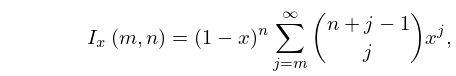
8.17.24 $$I_x(m,n)={(1-x)}^n\sum _{j=m}^{\mathrm{\infty }}\left(\genfrac{}{}{0.0pt}{}{n+j-1}{j}\right)x^j,$$ $m,n$ positive integers; .

ⓘ

Symbols:

$I_x(a,b)$: incomplete beta function, $\left(\genfrac{}{}{0.0pt}{}{m}{n}\right)$: binomial coefficient, $n$: nonnegative integer and $x$: variable

A&S Ref:

26.5.26 (The upper limit of summation has been corrected.)

Referenced by:

§8.17(i), Erratum (V1.0.5) for Chapters 8, 20, 36

Permalink:

http://dlmf.nist.gov/8.17.E24

Encodings:

pMML, png, TeX

Addition (effective with 1.0.5):

This equation is the same as Equation (26.5.26) of Abramowitz and Stegun (1964), except that the upper limit of the summation has been corrected to $\mathrm{\infty }$.

Suggested 2011-03-23 by Stephen Bourn

See also:

Annotations for §8.17(vii), §8.17 and Ch.8

…

30: 11.6 Asymptotic Expansions

… ►

$c_3(\lambda )=20{\lambda }^{-6}-4{\lambda }^{-4},$

…