special values of the variable

(0.005 seconds)

21—30 of 83 matching pages

21: 28.12 Definitions and Basic Properties

… ►

§28.12(i) Eigenvalues $\lambda_{\nu+2n}\left(q\right)$

… ► … ►As in §28.7 values of

q

for which (28.2.16) has simple roots

\lambda

are called normal values with respect to

\nu

. … ►If

q

is a normal value of the corresponding equation (28.2.16), then these functions are uniquely determined as analytic functions of

z

and

q

by the normalization …(28.12.10) is not valid for cuts on the real axis in the

q

-plane for special complex values of

\nu

; but it remains valid for small

q

; compare §28.7. …

22: 13.4 Integral Representations

… ►

13.4.1

{\mathbf{M}}\left(a,b,z\right)=\frac{1}{\Gamma\left(a\right)\Gamma\left(b-a% \right)}\int_{0}^{1}e^{zt}t^{a-1}(1-t)^{b-a-1}\,\mathrm{d}t,

\Re b>\Re a>0

ⓘ

Symbols:: $\Gamma\left(\NVar{z}\right)$ : gamma function, ${\mathbf{M}}\left(\NVar{a},\NVar{b},\NVar{z}\right)$ : Olver’s confluent hypergeometric function, $\,\mathrm{d}\NVar{x}$ : differential of $x$ , $\mathrm{e}$ : base of natural logarithm, $\int$ : integral, $\Re$ : real part and $z$ : complex variable
A&S Ref:: 13.2.1 (in different form)
Referenced by:: §13.10(v), §13.29(iii)
Permalink:: http://dlmf.nist.gov/13.4.E1
Encodings:: pMML, png, TeX
See also:: Annotations for §13.4(i), §13.4 and Ch.13

… ►The fractional powers are continuous and assume their principal values at

t=\alpha

. …At the point where the contour crosses the interval

(1,\infty)

t^{-b}

and the

{{}_{2}{\mathbf{F}}_{1}}

function assume their principal values; compare §§15.1 and 15.2(i). A special case is … ►Again,

t^{-c}

and the

{{}_{2}{\mathbf{F}}_{1}}

function assume their principal values where the contour intersects the positive real axis. …

23: 1.14 Integral Transforms

… ►The Fourier transform of a real- or complex-valued function

f(t)

is defined by … ►where the last integral denotes the Cauchy principal value (1.4.25). … ►Suppose

f(t)

is a real- or complex-valued function and

s

is a real or complex parameter. … ►The Mellin transform of a real- or complex-valued function

f(x)

is defined by … ►The Stieltjes transform of a real-valued function

f(t)

is defined by …

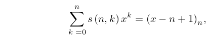
24: 26.8 Set Partitions: Stirling Numbers

… ►

26.8.7

\sum_{k=0}^{n}s\left(n,k\right)x^{k}={\left(x-n+1\right)_{n}},

ⓘ

Symbols:: ${\left(\NVar{a}\right)_{\NVar{n}}}$ : Pochhammer’s symbol (or shifted factorial), $s\left(\NVar{n},\NVar{k}\right)$ : Stirling number of the first kind, $x$ : real variable, $k$ : nonnegative integer and $n$ : nonnegative integer
A&S Ref:: 24.1.3 (in slightly different form)
Permalink:: http://dlmf.nist.gov/26.8.E7
Encodings:: pMML, png, TeX
Addition (effective with 1.1.2):: The Pochhammer symbol now links to its definition.
See also:: Annotations for §26.8(ii), §26.8 and Ch.26

… ►

26.8.10

\sum_{k=1}^{n}S\left(n,k\right){\left(x-k+1\right)_{k}}=x^{n},

ⓘ

Symbols:: ${\left(\NVar{a}\right)_{\NVar{n}}}$ : Pochhammer’s symbol (or shifted factorial), $S\left(\NVar{n},\NVar{k}\right)$ : Stirling number of the second kind, $x$ : real variable, $k$ : nonnegative integer and $n$ : nonnegative integer
A&S Ref:: 24.1.4
Referenced by:: §26.15
Permalink:: http://dlmf.nist.gov/26.8.E10
Encodings:: pMML, png, TeX
Addition (effective with 1.1.2):: The Pochhammer symbol now links to its definition.
See also:: Annotations for §26.8(ii), §26.8 and Ch.26

… ►

§26.8(iii) Special Values

►For

n\geq 1

, … ►

26.8.32

\Delta f(x)=f(x+1)-f(x);

ⓘ

Symbols:: $\Delta$ : forward difference operator and $x$ : real variable
Permalink:: http://dlmf.nist.gov/26.8.E32
Encodings:: pMML, png, TeX
See also:: Annotations for §26.8(v), §26.8 and Ch.26

…

25: 4.1 Special Notation

§4.1 Special Notation

►(For other notation see Notation for the Special Functions.) ► ►►►►

$k, m, n$	integers.
…
$x, y$	real variables.
$z=x+\mathrm{i}y$	complex variable.
…

…

26: 5.4 Special Values and Extrema

… ►

5.4.19

\psi\left(\frac{p}{q}\right)=-\gamma-\ln q-\frac{\pi}{2}\cot\left(\frac{\pi p}% {q}\right)+\frac{1}{2}\sum_{k=1}^{q-1}\cos\left(\frac{2\pi kp}{q}\right)\ln% \left(2-2\cos\left(\frac{2\pi k}{q}\right)\right).

ⓘ

Symbols:: $\gamma$ : Euler’s constant, $\pi$ : the ratio of the circumference of a circle to its diameter, $\cos\NVar{z}$ : cosine function, $\cot\NVar{z}$ : cotangent function, $\psi\left(\NVar{z}\right)$ : psi (or digamma) function, $\ln\NVar{z}$ : principal branch of logarithm function, $q$ : real or complex variable and $k$ : nonnegative integer
Referenced by:: §5.19(i), §5.4(ii)
Permalink:: http://dlmf.nist.gov/5.4.E19
Encodings:: pMML, png, TeX
See also:: Annotations for §5.4(ii), §5.4 and Ch.5

…

27: 36.12 Uniform Approximation of Integrals

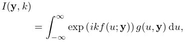
… ►In the cuspoid case (one integration variable) ►

36.12.1

I(\mathbf{y},k)=\int_{-\infty}^{\infty}\exp\left(ikf(u;\mathbf{y})\right)g(u,% \mathbf{y})\,\mathrm{d}u,

ⓘ

Defines:: $I(\mathbf{y},k)$ : oscillatory integral (locally)
Symbols:: $\,\mathrm{d}\NVar{x}$ : differential of $x$ , $\exp\NVar{z}$ : exponential function, $\mathrm{i}$ : imaginary unit, $\int$ : integral, $k$ : variable, $g(u,\mathbf{y})$ : function, $f(u,\mathbf{y})$ : function and $u(t;\mathbf{y})$ : mapping
Referenced by:: §36.13
Permalink:: http://dlmf.nist.gov/36.12.E1
Encodings:: pMML, png, TeX
See also:: Annotations for §36.12(i), §36.12 and Ch.36

… ►If

\ifrac{{\partial}^{K+2}f}{{\partial u}^{K+2}}<0

, then we may evaluate the complex conjugate of

I

for real values of

\mathbf{y}

and

g

, and obtain

I

by conjugation and analytic continuation. … ►

§36.12(ii) Special Case

►For

K=1

, with a single parameter

y

, let the two critical points of

f(u;y)

be denoted by

u_{\pm}(y)

, with

u_{+}>u_{-}

for those values of

y

for which these critical points are real. …

28: 14.1 Special Notation

§14.1 Special Notation

►(For other notation see Notation for the Special Functions.) ► ►►►

$x$ , $y$ , $\tau$	real variables.
$z=x+iy$	complex variable.
…

►Multivalued functions take their principal values (§4.2(i)) unless indicated otherwise. …

29: 10.2 Definitions

… ►

§10.2(ii) Standard Solutions

… ►The principal branch of

J_{\nu}\left(z\right)

corresponds to the principal value of

(\tfrac{1}{2}z)^{\nu}

(§4.2(iv)) and is analytic in the

z

-plane cut along the interval

(-\infty,0]

. … ►When

\nu

is an integer the right-hand side is replaced by its limiting value: … ►The principal branches correspond to principal values of the square roots in (10.2.5) and (10.2.6), again with a cut in the

z

-plane along the interval

(-\infty,0]

. … ► …

30: 19.2 Definitions