regular solutions

SearchAdvancedHelp

(0.001 seconds)

21—28 of 28 matching pages

21: 28.2 Definitions and Basic Properties

… ►This equation has regular singularities at 0 and 1, both with exponents 0 and $\frac{1}{2}$, and an irregular singular point at $\mathrm{\infty }$. … ►

§28.2(iv) Floquet Solutions

… ►The Fourier series of a Floquet solution …leads to a Floquet solution. … ►For the connection with the basic solutions in §28.2(ii), …

22: 16.8 Differential Equations

… ►If $z_0$ is not an ordinary point but ${(z-z_0)}^{n-j}{f}_j(z)$, $j=0,1,\mathrm{\dots },n-1$, are analytic at $z=z_0$, then $z_0$ is a regular singularity. … ►Equation (16.8.4) has a regular singularity at $z=0$, and an irregular singularity at $z=\mathrm{\infty }$, whereas (16.8.5) has regular singularities at $z=0$, $1$, and $\mathrm{\infty }$. … ►When no $b_j$ is an integer, and no two $b_j$ differ by an integer, a fundamental set of solutions of (16.8.3) is given by … ►When $p=q+1$, and no two $a_j$ differ by an integer, another fundamental set of solutions of (16.8.3) is given by … ►Thus in the case $p=q$ the regular singularities of the function on the left-hand side at $\alpha$ and $\mathrm{\infty }$ coalesce into an irregular singularity at $\mathrm{\infty }$. …

23: Bibliography L

… ►

The solutions of the Mathieu equation with a complex variable and at least one parameter large. Trans. Amer. Math. Soc. 36 (3), pp. 637–695.

ⓘ

External Links:

ISSN 0002-9947, FullText, MathReview Entry, ZentralBlatt

Referenced by:

§28.8(iv).

Encodings:

BibTeX

… ►

Exact operator solution of the Calogero-Sutherland model. Comm. Math. Phys. 178 (2), pp. 425–452.

ⓘ

Notes:

For a Maple implementation of the algorithm given in this paper for Jack and zonal polynomials see Zeilberger (website).

External Links:

ISSN 0010-3616, Link, MathReview (Kazuhiro Hikami), ZentralBlatt

Referenced by:

§35.12.

Encodings:

BibTeX

… ►

Generalized Riemann $\zeta$-function regularization and Casimir energy for a piecewise uniform string. Phys. Rev. D 44 (2), pp. 560–562.

ⓘ

External Links:

Document

Referenced by:

§24.18.

Encodings:

BibTeX

… ►

Well-posedness and blow-up solutions for an integrable nonlinearly dispersive model wave equation. J. Differential Equations 162 (1), pp. 27–63.

ⓘ

External Links:

ISSN 0022-0396, Document, MathReview (John Albert), ZentralBlatt

Referenced by:

§22.19(iii).

Encodings:

BibTeX

… ►

Numerical Solution of Linear Difference Equations. NBSIR Technical Report 80-1976, National Bureau of Standards, Gaithersburg, MD 20899.

ⓘ

Notes:

(Available from National Technical Information Service, Springfield, VA 22161.)

Referenced by:

§16.25, §3.6(vii).

Encodings:

BibTeX

…

24: 15.10 Hypergeometric Differential Equation

… ►

§15.10(i) Fundamental Solutions

… ►It has regular singularities at $z=0,1,\mathrm{\infty }$, with corresponding exponent pairs $\{0,1-c\}$, $\{0,c-a-b\}$, $\{a,b\}$, respectively. … ► ►

§15.10(ii) Kummer’s 24 Solutions and Connection Formulas

►The three pairs of fundamental solutions given by (15.10.2), (15.10.4), and (15.10.6) can be transformed into 18 other solutions by means of (15.8.1), leading to a total of 24 solutions known as Kummer’s solutions. …

25: 31.2 Differential Equations

… ►This equation has regular singularities at $0,1,a,\mathrm{\infty }$, with corresponding exponents $\{0,1-\gamma \}$, $\{0,1-\delta \}$, $\{0,1-ϵ\}$, $\{\alpha ,\beta \}$, respectively (§2.7(i)). All other homogeneous linear differential equations of the second order having four regular singularities in the extended complex plane, $ℂ\cup \{\mathrm{\infty }\}$, can be transformed into (31.2.1). … ► $w(z)=z^{1-\gamma }{w}_1(z)$ satisfies (31.2.1) if $w_1$ is a solution of (31.2.1) with transformed parameters $q_1=q+(a\delta +ϵ)(1-\gamma )$; ${\alpha }_1=\alpha +1-\gamma$, ${\beta }_1=\beta +1-\gamma$, ${\gamma }_1=2-\gamma$. Next, $w(z)={(z-1)}^{1-\delta }{w}_2(z)$ satisfies (31.2.1) if $w_2$ is a solution of (31.2.1) with transformed parameters $q_2=q+a\gamma (1-\delta )$; ${\alpha }_2=\alpha +1-\delta$, ${\beta }_2=\beta +1-\delta$, ${\delta }_2=2-\delta$. … ►If $\tilde{z}=\tilde{z}(z)$ is one of the $3!=6$ homographies that map $\mathrm{\infty }$ to $\mathrm{\infty }$, then $w(z)=\tilde{w}(\tilde{z})$ satisfies (31.2.1) if $\tilde{w}(\tilde{z})$ is a solution of (31.2.1) with $z$ replaced by $\tilde{z}$ and appropriately transformed parameters. …

26: 31.14 General Fuchsian Equation

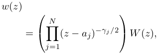
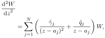
… ►The general second-order Fuchsian equation with $N+1$ regular singularities at $z=a_j$, $j=1,2,\mathrm{\dots },N$, and at $\mathrm{\infty }$, is given by … ►

31.14.3 $$w(z)=\left(\prod _{j=1}^N{(z-a_j)}^{-{\gamma }_j/2}\right)W(z),$$

ⓘ

Symbols:

$z$: complex variable, $\gamma$: real or complex parameter, $j$: nonnegative integer, $a$: complex parameter, $N+1$: number of singularities and $W(z)$: solution

Permalink:

http://dlmf.nist.gov/31.14.E3

Encodings:

pMML, png, TeX

See also:

Annotations for §31.14(i), §31.14(i), §31.14 and Ch.31

►

31.14.4 $$\frac{d^{2}W}{{dz}^2}=\sum _{j=1}^N\left(\frac{{\tilde{\gamma }}_j}{{(z-a_j)}^2}+\frac{{\tilde{q}}_j}{z-a_j}\right)W,$$ ${\sum }_{j=1}^N{\tilde{q}}_j=0$,

ⓘ

Defines:

$W(z)$: solution (locally)

Symbols:

$\frac{df}{dx}$: derivative of $f$ with respect to $x$ , $z$: complex variable, $\gamma$: real or complex parameter, $j$: nonnegative integer, $a$: complex parameter, $q$: real or complex parameter and $N+1$: number of singularities

Permalink:

http://dlmf.nist.gov/31.14.E4

Encodings:

pMML, png, TeX

See also:

Annotations for §31.14(i), §31.14(i), §31.14 and Ch.31

… ►An algorithm given in Kovacic (1986) determines if a given (not necessarily Fuchsian) second-order homogeneous linear differential equation with rational coefficients has solutions expressible in finite terms (Liouvillean solutions). The algorithm returns a list of solutions if they exist. …

27: 18.39 Applications in the Physical Sciences

… ►The solutions of (18.39.8) are subject to boundary conditions at $a$ and $b$. … ►The solutions (18.39.8) are called the stationary states as separation of variables in (18.39.9) yields solutions of form … ►Brief mention of non-unit normalized solutions in the case of mixed spectra appear, but as these solutions are not OP’s details appear elsewhere, as referenced. … ►Kuijlaars and Milson (2015, §1) refer to these, in this case complex zeros, as exceptional, as opposed to regular, zeros of the EOP’s, these latter belonging to the (real) orthogonality integration range. … ►The radial Coulomb wave functions $R_{n,l}(r)$, solutions of …

28: Bibliography G

… ►

The solution of Cauchy’s problem for two totally hyperbolic linear differential equations by means of Riesz integrals. Ann. of Math. (2) 48 (4), pp. 785–826.

ⓘ

External Links:

FullText, MathReview (E. T. Copson), ZentralBlatt

Referenced by:

§35.2, §35.3(ii).

Encodings:

BibTeX

… ►

Algorithm 292: Regular Coulomb wave functions. Comm. ACM 9 (11), pp. 793–795.

ⓘ

External Links:

ISSN 0001-0782, Document

Referenced by:

§33.26(ii).

Encodings:

BibTeX

… ►

Computing solutions of the modified Bessel differential equation for imaginary orders and positive arguments. ACM Trans. Math. Software 30 (2), pp. 145–158.

ⓘ

External Links:

ISSN 0098-3500, Document, MathReview, ZentralBlatt

Referenced by:

§10.74(viii).

Encodings:

BibTeX

… ►

Numerically satisfactory solutions of hypergeometric recursions. Math. Comp. 76 (259), pp. 1449–1468.

ⓘ

External Links:

ISSN 0025-5718, FullText, Document, MathReview Entry, ZentralBlatt

Referenced by:

§15.19(iv).

Encodings:

BibTeX

… ►

Computing the zeros and turning points of solutions of second order homogeneous linear ODEs. SIAM J. Numer. Anal. 41 (3), pp. 827–855.

ⓘ

External Links:

ISSN 0036-1429, Document, MathReview, ZentralBlatt

Referenced by:

§10.74(vi), §3.8(v).

Encodings:

BibTeX

…