region

SearchAdvancedHelp

(0.001 seconds)

11—20 of 60 matching pages

11: 25.10 Zeros

… ►In the region , called the critical strip, $\zeta \left(s\right)$ has infinitely many zeros, distributed symmetrically about the real axis and about the critical line $\mathrm{\Re }s=\frac{1}{2}$. … ►By comparing $N(T)$ with the number of sign changes of $Z(t)$ we can decide whether $\zeta \left(s\right)$ has any zeros off the line in this region. …

12: 9.16 Physical Applications

… ►The Airy functions constitute uniform approximations whose region of validity includes the turning point and its neighborhood. …

13: 9.17 Methods of Computation

… ►In the case of the Scorer functions, integration of the differential equation (9.12.1) is more difficult than (9.2.1), because in some regions stable directions of integration do not exist. …

14: 13.7 Asymptotic Expansions for Large Argument

… ►

13.7.2 $$𝐌(a,b,z)\sim \frac{{\mathrm{e}}^z{z}^{a-b}}{\mathrm{\Gamma }\left(a\right)}\sum _{s=0}^{\mathrm{\infty }}\frac{{\left(1-a\right)}_s{\left(b-a\right)}_s}{s!}{z}^{-s}+\frac{{\mathrm{e}}^{\pm \pi \mathrm{i}a}{z}^{-a}}{\mathrm{\Gamma }\left(b-a\right)}\sum _{s=0}^{\mathrm{\infty }}\frac{{\left(a\right)}_s{\left(a-b+1\right)}_s}{s!}{(-z)}^{-s},$$ $-\frac{1}{2}\pi +\delta \le \pm \mathrm{ph}z\le \frac{3}{2}\pi -\delta$,

ⓘ

Symbols:

$\mathrm{\Gamma }\left(z\right)$: gamma function, $𝐌(a,b,z)$: Olver’s confluent hypergeometric function, ${\left(a\right)}_n$: Pochhammer’s symbol (or shifted factorial), $\sim$: Poincaré asymptotic expansion, $\pi$: the ratio of the circumference of a circle to its diameter, $\mathrm{e}$: base of natural logarithm, $!$: factorial (as in $n!$), $\mathrm{i}$: imaginary unit, $\mathrm{ph}$: phase, $s$: nonnegative integer, $z$: complex variable and $\delta$: small positive constant

A&S Ref:

13.5.1 (with corrected region of validity)

Referenced by:

§13.2(iv), §13.7(ii), §13.9(i)

Permalink:

http://dlmf.nist.gov/13.7.E2

Encodings:

pMML, png, TeX

See also:

Annotations for §13.7(i), §13.7 and Ch.13

… ►

►►

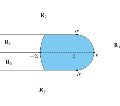
Figure 13.7.1: Regions ${\text{R}}_1$, ${\text{R}}_2$, ${\overline{\text{R}}}_2$, ${\text{R}}_3$, and ${\overline{\text{R}}}_3$ are the closures of the indicated unshaded regions bounded by the straight lines and circular arcs centered at the origin, with $r=|b-2a|$. Magnify

…

15: 33.12 Asymptotic Expansions for Large $\eta$

… ►

§33.12(i) Transition Region

…

16: 10.19 Asymptotic Expansions for Large Order

… ►

§10.19(iii) Transition Region

…

17: 18.24 Hahn Class: Asymptotic Approximations

… ►When the parameters $\alpha$ and $\beta$ are fixed and the ratio $n/N=c$ is a constant in the interval (0,1), uniform asymptotic formulas (as $n\to \mathrm{\infty }$ ) of the Hahn polynomials $Q_n(z;\alpha ,\beta ,N)$ can be found in Lin and Wong (2013) for $z$ in three overlapping regions, which together cover the entire complex plane. …

18: 35.2 Laplace Transform

… ►Then (35.2.1) converges absolutely on the region $\mathrm{\Re }\left(𝐙\right)>{𝐗}_0$, and $g(𝐙)$ is a complex analytic function of all elements $z_{j,k}$ of $𝐙$. …

19: 9.2 Differential Equation

… ►Table 9.2.1 lists numerically satisfactory pairs of solutions of (9.2.1) for the stated intervals or regions; compare §2.7(iv). ►

Table 9.2.1: Numerically satisfactory pairs of solutions of Airy’s equation.

► ►►

Pair	Interval or Region
…

►

…

20: 18.40 Methods of Computation

… ►The question is then: how is this possible given only $F_N(z)$, rather than $F(z)$ itself? $F_N(z)$ often converges to smooth results for $z$ off the real axis for $\mathrm{\Im }z$ at a distance greater than the pole spacing of the $x_n$, this may then be followed by approximate numerical analytic continuation via fitting to lower order continued fractions (either Padé, see §3.11(iv), or pointwise continued fraction approximants, see Schlessinger (1968, Appendix)), to $F_N(z)$ and evaluating these on the real axis in regions of higher pole density that those of the approximating function. … ►

►►

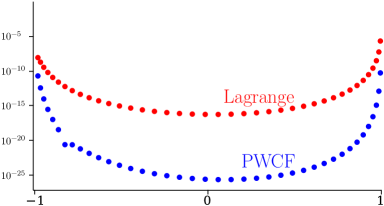
Figure 18.40.2: Derivative Rule inversions for $w^{\mathrm{RCP}}(x)$ carried out via Lagrange and PWCF interpolations. …For the derivative rule Lagrange interpolation (red points) gives $\sim 15$ digits in the central region, while PWCF interpolation (blue points) gives $\sim 25$. Magnify

…