q-multinomial coefficient

SearchAdvancedHelp

(0.002 seconds)

21—30 of 241 matching pages

21: 7.24 Approximations

… ►

Luke (1969b, pp. 323–324) covers $\frac{1}{2}\sqrt{\pi }\mathrm{erf}x$ and ${\mathrm{e}}^{x^2}F\left(x\right)$ for $-3\le x\le 3$ (the Chebyshev coefficients are given to 20D); $\sqrt{\pi }x{\mathrm{e}}^{x^2}\mathrm{erfc}x$ and $2xF\left(x\right)$ for $x\ge 3$ (the Chebyshev coefficients are given to 20D and 15D, respectively). Coefficients for the Fresnel integrals are given on pp. 328–330 (20D).

►

Bulirsch (1967) provides Chebyshev coefficients for the auxiliary functions $\mathrm{f}\left(x\right)$ and $\mathrm{g}\left(x\right)$ for $x\ge 3$ (15D).

►

Schonfelder (1978) gives coefficients of Chebyshev expansions for $x^{-1}\mathrm{erf}x$ on $0\le x\le 2$, for $x{\mathrm{e}}^{x^2}\mathrm{erfc}x$ on $[2,\mathrm{\infty })$, and for ${\mathrm{e}}^{x^2}\mathrm{erfc}x$ on $[0,\mathrm{\infty })$ (30D).

►

Shepherd and Laframboise (1981) gives coefficients of Chebyshev series for $(1+2x){\mathrm{e}}^{x^2}\mathrm{erfc}x$ on $(0,\mathrm{\infty })$ (22D).

…

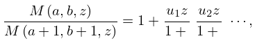
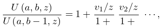
22: 13.5 Continued Fractions

… ►

13.5.1 $$\frac{M(a,b,z)}{M(a+1,b+1,z)}=1+\frac{u_{1}z}{1+}\frac{u_{2}z}{1+}\mathrm{\cdots },$$

ⓘ

Symbols:

$M(a,b,z)$: $={}_1{}^{}F_1^{}(a;b;z)$ Kummer confluent hypergeometric function, $z$: complex variable and $u_n$: continued fraction coefficients

Referenced by:

§13.31(ii)

Permalink:

http://dlmf.nist.gov/13.5.E1

Encodings:

pMML, png, TeX

See also:

Annotations for §13.5 and Ch.13

… ►

13.5.3 $$\frac{U(a,b,z)}{U(a,b-1,z)}=1+\frac{v_1/z}{1+}\frac{v_2/z}{1+}\mathrm{\cdots },$$

ⓘ

Symbols:

$U(a,b,z)$: Kummer confluent hypergeometric function, $z$: complex variable and $v_n$: continued fraction coefficients

Permalink:

http://dlmf.nist.gov/13.5.E3

Encodings:

pMML, png, TeX

See also:

Annotations for §13.5 and Ch.13

…

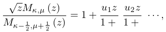
23: 13.17 Continued Fractions

… ►

13.17.1 $$\frac{\sqrt{z}{M}_{\kappa ,\mu }\left(z\right)}{M_{\kappa -\frac{1}{2},\mu +\frac{1}{2}}\left(z\right)}=1+\frac{u_{1}z}{1+}\frac{u_{2}z}{1+}\mathrm{\cdots },$$

ⓘ

Symbols:

$M_{\kappa ,\mu }\left(z\right)$: Whittaker confluent hypergeometric function, $z$: complex variable and $u_n$: continued fraction coefficients

Permalink:

http://dlmf.nist.gov/13.17.E1

Encodings:

pMML, png, TeX

See also:

Annotations for §13.17 and Ch.13

… ►

13.17.3 $$\frac{W_{\kappa ,\mu }\left(z\right)}{\sqrt{z}{W}_{\kappa -\frac{1}{2},\mu -\frac{1}{2}}\left(z\right)}=1+\frac{v_1/z}{1+}\frac{v_2/z}{1+}\mathrm{\cdots },$$

ⓘ

Symbols:

$W_{\kappa ,\mu }\left(z\right)$: Whittaker confluent hypergeometric function, $z$: complex variable and $v_n$: continued fraction coefficients

Permalink:

http://dlmf.nist.gov/13.17.E3

Encodings:

pMML, png, TeX

See also:

Annotations for §13.17 and Ch.13

…

24: 18.3 Definitions

… ►

Table 18.3.1: Orthogonality properties for classical OP’s: intervals, weight functions, standardizations, leading coefficients, and parameter constraints. …

► ►►

Name	$p_n(x)$	$(a,b)$	$w(x)$	$h_n$	$k_n$	${\tilde{k}}_n/k_n$	Constraints
…

►

… ►For explicit power series coefficients up to $n=12$ for these polynomials and for coefficients up to $n=6$ for Jacobi and ultraspherical polynomials see Abramowitz and Stegun (1964, pp. 793–801). …

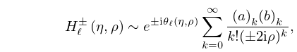
25: 33.11 Asymptotic Expansions for Large $\rho$

… ►

33.11.1 $$H_{\mathrm{\ell }}^{\pm }(\eta ,\rho )\sim {\mathrm{e}}^{\pm \mathrm{i}{\theta }_{\mathrm{\ell }}(\eta ,\rho )}\sum _{k=0}^{\mathrm{\infty }}\frac{{\left(a\right)}_k{\left(b\right)}_k}{k!{(\pm 2\mathrm{i}\rho )}^k},$$

ⓘ

Symbols:

${\theta }_{\mathrm{\ell }}(\eta ,\rho )$: phase of Coulomb functions, ${\left(a\right)}_n$: Pochhammer’s symbol (or shifted factorial), $\sim$: Poincaré asymptotic expansion, $\mathrm{e}$: base of natural logarithm, $!$: factorial (as in $n!$), $\mathrm{i}$: imaginary unit, $H_{\mathrm{\ell }}^{\pm }(\eta ,\rho )$: irregular Coulomb radial functions, $k$: nonnegative integer, $\mathrm{\ell }$: nonnegative integer, $\rho$: nonnegative real variable, $\eta$: real parameter, $a$: coefficient and $b$: coefficient

A&S Ref:

14.5.9

Referenced by:

Erratum (V1.0.19) for Equation (33.11.1), Erratum (V1.0.22) for Equation (33.11.1)

Permalink:

http://dlmf.nist.gov/33.11.E1

Encodings:

pMML, png, TeX

Errata (effective with 1.0.22):

Previously this formula was expressed as an equality. Since this formula expresses an asymptotic expansion, it has been corrected by using instead an $\sim$ relation.

Reported 2019-01-29 by Gergő Nemes

Errata (effective with 1.0.19):

Originally the factor in the denominator on the right-hand side was written incorrectly as ${(\mp 2\mathrm{i}\rho )}^k$. This has been corrected to ${(\pm 2\mathrm{i}\rho )}^k$.

Reported 2018-05-15 by Ian Thompson

See also:

Annotations for §33.11 and Ch.33

…

26: 9.19 Approximations

… ►

Prince (1975) covers $\mathrm{Ai}\left(x\right)$, ${\mathrm{Ai}}^{\prime }\left(x\right)$, $\mathrm{Bi}\left(x\right)$, ${\mathrm{Bi}}^{\prime }\left(x\right)$. The Chebyshev coefficients are given to 10-11D. Fortran programs are included. See also Razaz and Schonfelder (1981).

►

Németh (1992, Chapter 8) covers $\mathrm{Ai}\left(x\right)$, ${\mathrm{Ai}}^{\prime }\left(x\right)$, $\mathrm{Bi}\left(x\right)$, ${\mathrm{Bi}}^{\prime }\left(x\right)$, and integrals ${\int }_0^x\mathrm{Ai}\left(t\right)dt$, ${\int }_0^x\mathrm{Bi}\left(t\right)dt$, ${\int }_0^x{\int }_0^v\mathrm{Ai}\left(t\right)dtdv$, ${\int }_0^x{\int }_0^v\mathrm{Bi}\left(t\right)dtdv$ (see also (9.10.20) and (9.10.21)). The Chebyshev coefficients are given to 15D. Chebyshev coefficients are also given for expansions of the second and higher (real) zeros of $\mathrm{Ai}\left(x\right)$, ${\mathrm{Ai}}^{\prime }\left(x\right)$, $\mathrm{Bi}\left(x\right)$, ${\mathrm{Bi}}^{\prime }\left(x\right)$, again to 15D.

►

Razaz and Schonfelder (1980) covers $\mathrm{Ai}\left(x\right)$, ${\mathrm{Ai}}^{\prime }\left(x\right)$, $\mathrm{Bi}\left(x\right)$, ${\mathrm{Bi}}^{\prime }\left(x\right)$. The Chebyshev coefficients are given to 30D.

… ►

Corless et al. (1992) describe a method of approximation based on subdividing $ℂ$ into a triangular mesh, with values of $\mathrm{Ai}\left(z\right)$, ${\mathrm{Ai}}^{\prime }\left(z\right)$ stored at the nodes. $\mathrm{Ai}\left(z\right)$ and ${\mathrm{Ai}}^{\prime }\left(z\right)$ are then computed from Taylor-series expansions centered at one of the nearest nodes. The Taylor coefficients are generated by recursion, starting from the stored values of $\mathrm{Ai}\left(z\right)$, ${\mathrm{Ai}}^{\prime }\left(z\right)$ at the node. Similarly for $\mathrm{Bi}\left(z\right)$, ${\mathrm{Bi}}^{\prime }\left(z\right)$.

… ►

MacLeod (1994) supplies Chebyshev-series expansions to cover $\mathrm{Gi}\left(x\right)$ for and $\mathrm{Hi}\left(x\right)$ for . The Chebyshev coefficients are given to 20D.

27: 29.7 Asymptotic Expansions

… ►

29.7.1 $$a_{\nu }^m\left(k^2\right)\sim p\kappa -{\tau }_0-{\tau }_1{\kappa }^{-1}-{\tau }_2{\kappa }^{-2}-\mathrm{\cdots },$$

ⓘ

Symbols:

$a_{\nu }^n\left(k^2\right)$: eigenvalues of Lamé’s equation, $\sim$: Poincaré asymptotic expansion, $m$: nonnegative integer, $p$: nonnegative integer, $k$: real parameter, $\nu$: real parameter, $\kappa$ and ${\tau }_j$: coefficients

Permalink:

http://dlmf.nist.gov/29.7.E1

Encodings:

pMML, png, TeX

See also:

Annotations for §29.7(i), §29.7 and Ch.29

… ►

29.7.3 $${\tau }_0=\frac{1}{2^3}(1+k^2)(1+p^2),$$

ⓘ

Symbols:

$p$: nonnegative integer, $k$: real parameter and ${\tau }_j$: coefficients

Permalink:

http://dlmf.nist.gov/29.7.E3

Encodings:

pMML, png, TeX

See also:

Annotations for §29.7(i), §29.7 and Ch.29

►

29.7.4 $${\tau }_1=\frac{p}{2^6}({(1+k^2)}^2(p^2+3)-4k^2(p^2+5)).$$

ⓘ

Symbols:

$p$: nonnegative integer, $k$: real parameter and ${\tau }_j$: coefficients

Permalink:

http://dlmf.nist.gov/29.7.E4

Encodings:

pMML, png, TeX

See also:

Annotations for §29.7(i), §29.7 and Ch.29

… ►

29.7.6 $${\tau }_2=\frac{1}{2^{10}}(1+k^2){(1-k^2)}^2(5p^4+34p^2+9),$$

ⓘ

Symbols:

$p$: nonnegative integer, $k$: real parameter and ${\tau }_j$: coefficients

Permalink:

http://dlmf.nist.gov/29.7.E6

Encodings:

pMML, png, TeX

See also:

Annotations for §29.7(i), §29.7 and Ch.29

►

29.7.7 $${\tau }_3=\frac{p}{2^{14}}({(1+k^2)}^4(33p^4+410p^2+405)-24k^2{(1+k^2)}^2(7p^4+90p^2+95)+16k^4(9p^4+130p^2+173)),$$

ⓘ

Symbols:

$p$: nonnegative integer, $k$: real parameter and ${\tau }_j$: coefficients

Permalink:

http://dlmf.nist.gov/29.7.E7

Encodings:

pMML, png, TeX

See also:

Annotations for §29.7(i), §29.7 and Ch.29

…

28: 3.6 Linear Difference Equations

… ►

3.6.1 $$a_n{w}_{n+1}-b_n{w}_n+c_n{w}_{n-1}=d_n,$$

ⓘ

Defines:

$a_n$: coefficient (locally), $b_n$: coefficient (locally), $c_n$: coefficient (locally) and $d_n$: coefficient (locally)

Symbols:

$w_n$: sequence

Referenced by:

§3.6(iv), §3.6(v)

Permalink:

http://dlmf.nist.gov/3.6.E1

Encodings:

pMML, png, TeX

See also:

Annotations for §3.6(i), §3.6 and Ch.3

… ►

3.6.2 $$a_n{\mathrm{\Delta }}^2{w}_{n-1}+(2a_n-b_n)\mathrm{\Delta }{w}_{n-1}+(a_n-b_n+c_n)w_{n-1}=d_n,$$

ⓘ

Symbols:

$\mathrm{\Delta }$: forward difference operator, $w_n$: sequence, $a_n$: coefficient, $b_n$: coefficient, $c_n$: coefficient and $d_n$: coefficient

Permalink:

http://dlmf.nist.gov/3.6.E2

Encodings:

pMML, png, TeX

See also:

Annotations for §3.6(i), §3.6 and Ch.3

… ►

3.6.3 $$a_n{w}_{n+1}-b_n{w}_n+c_n{w}_{n-1}=0,$$

ⓘ

Symbols:

$w_n$: sequence, $a_n$: coefficient, $b_n$: coefficient and $c_n$: coefficient

Referenced by:

§3.6(ii), §3.6(ii), §3.6(v), §3.6(v)

Permalink:

http://dlmf.nist.gov/3.6.E3

Encodings:

pMML, png, TeX

See also:

Annotations for §3.6(ii), §3.6 and Ch.3

… ►

3.6.8 $$a_n{e}_n=c_n{e}_{n-1}-d_n{p}_n,$$

ⓘ

Defines:

$e_n$: sequence (locally)

Symbols:

$p_n$: solutions, $a_n$: coefficient, $c_n$: coefficient and $d_n$: coefficient

Permalink:

http://dlmf.nist.gov/3.6.E8

Encodings:

pMML, png, TeX

See also:

Annotations for §3.6(v), §3.6 and Ch.3

… ►

3.6.17 $$a_n{w}_{n+1}-b_n{w}_n=d_n.$$

ⓘ

Symbols:

$w_n$: sequence, $a_n$: coefficient, $b_n$: coefficient and $d_n$: coefficient

Permalink:

http://dlmf.nist.gov/3.6.E17

Encodings:

pMML, png, TeX

See also:

Annotations for §3.6(vii), §3.6 and Ch.3

…

29: 24.5 Recurrence Relations

… ►

24.5.1 $$\sum _{k=0}^{n-1}\left(\genfrac{}{}{0pt}{}{n}{k}\right)B_k\left(x\right)=n{x}^{n-1},$$ $n=2,3,\mathrm{\dots }$,

ⓘ

Symbols:

$B_n\left(x\right)$: Bernoulli polynomials, $\left(\genfrac{}{}{0.0pt}{}{m}{n}\right)$: binomial coefficient, $k$: integer, $n$: integer and $x$: real or complex

Permalink:

http://dlmf.nist.gov/24.5.E1

Encodings:

pMML, png, TeX

See also:

Annotations for §24.5(i), §24.5 and Ch.24

►

24.5.2 $$\sum _{k=0}^n\left(\genfrac{}{}{0pt}{}{n}{k}\right)E_k\left(x\right)+E_n\left(x\right)=2x^n,$$ $n=1,2,\mathrm{\dots }$.

ⓘ

Symbols:

$E_n\left(x\right)$: Euler polynomials, $\left(\genfrac{}{}{0.0pt}{}{m}{n}\right)$: binomial coefficient, $k$: integer, $n$: integer and $x$: real or complex

Permalink:

http://dlmf.nist.gov/24.5.E2

Encodings:

pMML, png, TeX

See also:

Annotations for §24.5(i), §24.5 and Ch.24

►

24.5.3 $$\sum _{k=0}^{n-1}\left(\genfrac{}{}{0pt}{}{n}{k}\right)B_k=0,$$ $n=2,3,\mathrm{\dots }$,

ⓘ

Symbols:

$B_n$: Bernoulli numbers, $\left(\genfrac{}{}{0.0pt}{}{m}{n}\right)$: binomial coefficient, $k$: integer and $n$: integer

Referenced by:

§24.19(i)

Permalink:

http://dlmf.nist.gov/24.5.E3

Encodings:

pMML, png, TeX

See also:

Annotations for §24.5(i), §24.5 and Ch.24

►

24.5.4 $$\sum _{k=0}^n\left(\genfrac{}{}{0pt}{}{2n}{2k}\right)E_{2k}=0,$$ $n=1,2,\mathrm{\dots }$,

ⓘ

Symbols:

$E_n$: Euler numbers, $\left(\genfrac{}{}{0.0pt}{}{m}{n}\right)$: binomial coefficient, $k$: integer and $n$: integer

Referenced by:

§24.19(i)

Permalink:

http://dlmf.nist.gov/24.5.E4

Encodings:

pMML, png, TeX

See also:

Annotations for §24.5(i), §24.5 and Ch.24

►

24.5.5 $$\sum _{k=0}^n\left(\genfrac{}{}{0pt}{}{n}{k}\right)2^k{E}_{n-k}+E_n=2.$$

ⓘ

Symbols:

$E_n$: Euler numbers, $\left(\genfrac{}{}{0.0pt}{}{m}{n}\right)$: binomial coefficient, $k$: integer and $n$: integer

Permalink:

http://dlmf.nist.gov/24.5.E5

Encodings:

pMML, png, TeX

See also:

Annotations for §24.5(i), §24.5 and Ch.24

…

30: 2.2 Transcendental Equations

… ►In place of (2.2.1) assume that ►

2.2.7 $$f(x)\sim x+f_0+f_1{x}^{-1}+f_2{x}^{-2}+\mathrm{\cdots },$$ $x\to \mathrm{\infty }$.

ⓘ

Symbols:

$\sim$: Poincaré asymptotic expansion, $f(x)$: function and $f_s$: coefficients

Permalink:

http://dlmf.nist.gov/2.2.E7

Encodings:

pMML, png, TeX

See also:

Annotations for §2.2, §2.2 and Ch.2

… ►

2.2.8 $$x\sim y-F_0-F_1{y}^{-1}-F_2{y}^{-2}-\mathrm{\cdots },$$ $y\to \mathrm{\infty }$,

ⓘ

Symbols:

$\sim$: Poincaré asymptotic expansion, $y$: root and $F_s$: coefficients

Permalink:

http://dlmf.nist.gov/2.2.E8

Encodings:

pMML, png, TeX

See also:

Annotations for §2.2, §2.2 and Ch.2

►where $F_0=f_0$ and $s{F}_s$ ($s\ge 1$) is the coefficient of $x^{-1}$ in the asymptotic expansion of ${(f(x))}^s$ (Lagrange’s formula for the reversion of series). …