q-Askey scheme

SearchAdvancedHelp

(0.001 seconds)

1—10 of 31 matching pages

1: Howard S. Cohl

… ►His research interests include fundamental solutions of linear partial differential equations on Riemannian manifolds, associated Legendre and Jacobi functions, generalized and basic hypergeometric functions, eigenfunction expansions in separable coordinate systems, generating functions, $q$-series, and orthogonal polynomials in the Askey and $q$-Askey schemes. …

2: 1.11 Zeros of Polynomials

… ►

Horner’s Scheme

… ►

Extended Horner Scheme

…

3: 7.22 Methods of Computation

… ►The recursion scheme given by (7.18.1) and (7.18.7) can be used for computing ${\mathrm{i}}^n\mathrm{erfc}\left(x\right)$. …

4: 37.19 Other Orthogonal Polynomials of $d$ Variables

… ► … ►Just as the classical OPs fit into the Askey scheme (see §18.19 and Figure 18.21.1) with Wilson and Racah polynomials on top, the Jacobi polynomials on the simplex fit into a scheme of OPs defined as products of one-variable OPs belonging to the Askey scheme by formulas somewhat resembling (37.14.7). However, when the one-variable OPs are taken from a higher level in the Askey scheme, the analogues of the denominators in the arguments in (37.14.7) will be parameters depending on $x_{\mathrm{\ell }}$ variables. … ►Starting from OPs in the $q$-Askey scheme (see §18.27(i)), similar constructions of $d$-variable OPs can be made. …

5: 8.25 Methods of Computation

… ►Stable recursive schemes for the computation of $E_p\left(x\right)$ are described in Miller (1960) for $x>0$ and integer $p$. …

6: 16.24 Physical Applications

… ►The coefficients of transformations between different coupling schemes of three angular momenta are related to the Wigner $\mathit{6}j$ symbols. …

7: Richard A. Askey

… ►Published in 1985 in the Memoirs of the American Mathematical Society, it also introduced the directed graph of hypergeometric orthogonal polynomials commonly known as the Askey scheme. …

8: 6.20 Approximations

… ►

Luke (1969b, p. 25) gives a Chebyshev expansion near infinity for the confluent hypergeometric $U$-function (§13.2(i)) from which Chebyshev expansions near infinity for $E_1\left(z\right)$, $\mathrm{f}\left(z\right)$, and $\mathrm{g}\left(z\right)$ follow by using (6.11.2) and (6.11.3). Luke also includes a recursion scheme for computing the coefficients in the expansions of the $U$ functions. If the scheme can be used in backward direction.

…

9: 18.21 Hahn Class: Interrelations

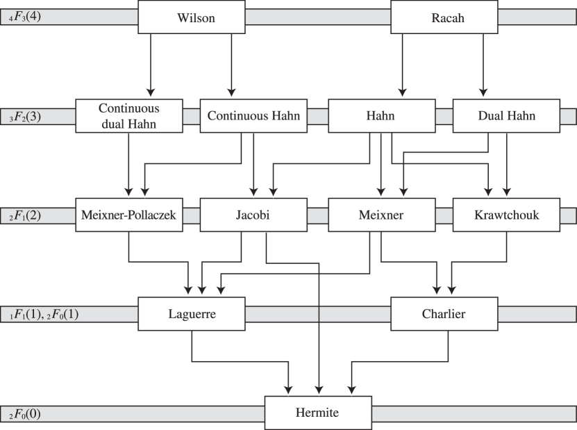
… ►A graphical representation of limits in §§18.7(iii), 18.21(ii), and 18.26(ii) is provided by the Askey scheme depicted in Figure 18.21.1. ►

►►

Figure 18.21.1: Askey scheme. …It increases by one for each row ascended in the scheme, culminating with four free real parameters for the Wilson and Racah polynomials. … Magnify

10: About Color Map

… ►The four color scheme quickly indicates in which quadrant $z$ lies: the colors blue, green, red and yellow are used to indicate the first, second, third and fourth quadrants, respectively. …