poles

SearchAdvancedHelp

(0.000 seconds)

31—40 of 60 matching pages

31: 25.15 Dirichlet $L$-functions

… ►For the principal character ${\chi }_1(modk)$, $L(s,{\chi }_1)$ is analytic everywhere except for a simple pole at $s=1$ with residue $\varphi \left(k\right)/k$, where $\varphi \left(k\right)$ is Euler’s totient function (§27.2). …

32: 2.5 Mellin Transform Methods

… ►The sum in (2.5.6) is taken over all poles of $x^{-z}ℳf\left(1-z\right)ℳh\left(z\right)$ in the strip , and it provides the asymptotic expansion of $I(x)$ for small values of $x$. … ►In the half-plane $\mathrm{\Re }z>\max (0,-2\nu )$, the product $ℳf\left(1-z\right)ℳh\left(z\right)$ has a pole of order two at each positive integer, and … ►Furthermore, $ℳf_1\left(z\right)$ can be continued analytically to a meromorphic function on the entire $z$-plane, whose singularities are simple poles at $-{\alpha }_s$, $s=0,1,2,\mathrm{\dots }$, with principal part … ►Similarly, if $\kappa =0$ in (2.5.18), then $ℳh_2\left(z\right)$ can be continued analytically to a meromorphic function on the entire $z$-plane with simple poles at ${\beta }_s$, $s=0,1,2,\mathrm{\dots }$, with principal part … ►Similarly, since $ℳh_2\left(z\right)$ can be continued analytically to a meromorphic function (when $\kappa =0$) or to an entire function (when $\kappa \ne 0$), we can choose $\rho$ so that $ℳh_2\left(z\right)$ has no poles in . …

33: 2.4 Contour Integrals

… ►For a coalescing saddle point and a pole see Wong (1989, Chapter 7) and van der Waerden (1951); in this case the uniform approximants are complementary error functions. … ►For a coalescing saddle point, a pole, and a branch point see Ciarkowski (1989). …

34: 10.32 Integral Representations

… ►In (10.32.14) the integration contour separates the poles of $\mathrm{\Gamma }\left(t\right)$ from the poles of $\mathrm{\Gamma }\left(\frac{1}{2}-t-\nu \right)\mathrm{\Gamma }\left(\frac{1}{2}-t+\nu \right)$. …

35: 15.6 Integral Representations

… ►In (15.6.6) the integration contour separates the poles of $\mathrm{\Gamma }\left(a+t\right)$ and $\mathrm{\Gamma }\left(b+t\right)$ from those of $\mathrm{\Gamma }\left(-t\right)$, and ${(-z)}^t$ has its principal value. ►In (15.6.7) the integration contour separates the poles of $\mathrm{\Gamma }\left(a+t\right)$ and $\mathrm{\Gamma }\left(b+t\right)$ from those of $\mathrm{\Gamma }\left(c-a-b-t\right)$ and $\mathrm{\Gamma }\left(-t\right)$, and ${(1-z)}^t$ has its principal value. …

36: 8.2 Definitions and Basic Properties

… ►When $z\ne 0$, $\mathrm{\Gamma }(a,z)$ is an entire function of $a$, and $\gamma (a,z)$ is meromorphic with simple poles at $a=-n$, $n=0,1,2,\mathrm{\dots }$, with residue ${(-1)}^n/n!$. …

37: 11.5 Integral Representations

… ►In (11.5.8) and (11.5.9) the path of integration separates the poles of the integrand at $s=0,1,2,\mathrm{\dots }$ from those at $s=-1,-2,-3,\mathrm{\dots }$. …

38: 14.19 Toroidal (or Ring) Functions

… ►

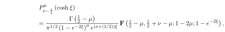
14.19.2 $$P_{\nu -\frac{1}{2}}^{\mu }\left(\cosh \xi \right)=\frac{\mathrm{\Gamma }\left(\frac{1}{2}-\mu \right)}{{\pi }^{1/2}{\left(1-{\mathrm{e}}^{-2\xi }\right)}^{\mu }{\mathrm{e}}^{(\nu +(1/2))\xi }}𝐅(\frac{1}{2}-\mu ,\frac{1}{2}+\nu -\mu ;1-2\mu ;1-{\mathrm{e}}^{-2\xi }),$$ $\mu \ne \frac{1}{2},\frac{3}{2},\frac{5}{2},\mathrm{\dots }$.

ⓘ

Symbols:

$\mathrm{\Gamma }\left(z\right)$: gamma function, $P_{\nu }^{\mu }\left(z\right)$: associated Legendre function of the first kind, $\pi$: the ratio of the circumference of a circle to its diameter, $\mathrm{e}$: base of natural logarithm, $\cosh z$: hyperbolic cosine function, $𝐅(a,b;c;z)$ or $𝐅(\genfrac{}{}{0pt}{}{a,b}{c};z)$: $={}_2{}^{}𝐅_1^{}(a,b;c;z)$ Olver’s hypergeometric function, $\mu$: general order, $\nu$: general degree and $\xi >0$: variable

Referenced by:

§14.19(ii), Erratum (V1.0.1) for Equation (14.19.2)

Permalink:

http://dlmf.nist.gov/14.19.E2

Encodings:

pMML, png, TeX

Errata (effective with 1.0.1):

Originally the argument to $𝐅$ was incorrect and the condition on $\mu$ too weak:

$$P_{\nu -\frac{1}{2}}^{\mu }\left(\cosh \xi \right)=\frac{\mathrm{\Gamma }\left(1-2\mu \right)2^{2\mu }}{\mathrm{\Gamma }\left(1-\mu \right){\left(1-{\mathrm{e}}^{-2\xi }\right)}^{\mu }{\mathrm{e}}^{(\nu +(1/2))\xi }}𝐅(\frac{1}{2}-\mu ,\frac{1}{2}+\nu -\mu ;1-2\mu ;{\mathrm{e}}^{-2\xi }),$$ $\mu \ne \frac{1}{2}$.

Also, the factor multiplying $𝐅$ was rewritten to clarify the poles, which determine the correct condition on $\mu$.

Reported 2010-11-02 by Alvaro Valenzuela

See also:

Annotations for §14.19(ii), §14.19 and Ch.14

…

39: 15.2 Definitions and Analytical Properties

… ►The same properties hold for $F(a,b;c;z)$, except that as a function of $c$, $F(a,b;c;z)$ in general has poles at $c=0,-1,-2,\mathrm{\dots }$. …

40: 16.5 Integral Representations and Integrals

… ►where the contour of integration separates the poles of $\mathrm{\Gamma }\left(a_k+s\right)$, $k=1,\mathrm{\dots },p$, from those of $\mathrm{\Gamma }\left(-s\right)$. …