point at infinity

SearchAdvancedHelp

(0.005 seconds)

11—20 of 77 matching pages

11: 4.13 Lambert $W$-Function

… ► $W_0\left(z\right)$ is a single-valued analytic function on $ℂ\setminus (-\mathrm{\infty },-{\mathrm{e}}^{-1}]$, real-valued when $z>-{\mathrm{e}}^{-1}$, and has a square root branch point at $z=-{\mathrm{e}}^{-1}$. …The other branches $W_k\left(z\right)$ are single-valued analytic functions on $ℂ\setminus (-\mathrm{\infty },0]$, have a logarithmic branch point at $z=0$, and, in the case $k=\pm 1$, have a square root branch point at $z=-{\mathrm{e}}^{-1}\mp 0\mathrm{i}$ respectively. …

12: 13.14 Definitions and Basic Properties

… ►In general $M_{\kappa ,\mu }\left(z\right)$ and $W_{\kappa ,\mu }\left(z\right)$ are many-valued functions of $z$ with branch points at $z=0$ and $z=\mathrm{\infty }$. …

13: 33.2 Definitions and Basic Properties

… ►

§33.2(i) Coulomb Wave Equation

… ►This differential equation has a regular singularity at $\rho =0$ with indices $\mathrm{\ell }+1$ and $-\mathrm{\ell }$, and an irregular singularity of rank 1 at $\rho =\mathrm{\infty }$ (§§2.7(i), 2.7(ii)). There are two turning points, that is, points at which $d^{2}w/{d\rho }^2=0$ (§2.8(i)). … ►The function $F_{\mathrm{\ell }}(\eta ,\rho )$ is recessive (§2.7(iii)) at $\rho =0$, and is defined by … ► $F_{\mathrm{\ell }}(\eta ,\rho )$ is a real and analytic function of $\rho$ on the open interval , and also an analytic function of $\eta$ when . …

14: 33.14 Definitions and Basic Properties

… ►

§33.14(i) Coulomb Wave Equation

… ►Again, there is a regular singularity at $r=0$ with indices $\mathrm{\ell }+1$ and $-\mathrm{\ell }$, and an irregular singularity of rank 1 at $r=\mathrm{\infty }$. When $ϵ>0$ the outer turning point is given by … ►The function $f(ϵ,\mathrm{\ell };r)$ is recessive (§2.7(iii)) at $r=0$, and is defined by … ► $f(ϵ,\mathrm{\ell };r)$ is real and an analytic function of $r$ in the interval , and it is also an analytic function of $ϵ$ when . …

15: 18.39 Applications in the Physical Sciences

… ►An important, and perhaps unexpected, feature of the EOP’s is now pointed out by noting that for 1D Schrödinger operators, or equivalent Sturm-Liouville ODEs, having discrete spectra with $L^2$ eigenfunctions vanishing at the end points, in this case $\pm \mathrm{\infty }$ see Simon (2005c, Theorem 3.3, p. 35), such eigenfunctions satisfy the Sturm oscillation theorem. … ►

►►

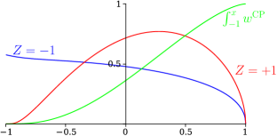
Figure 18.39.2: Coulomb–Pollaczek weight functions, $x\in [-1,1]$, (18.39.50) for $s=10$, $l=0$, and $Z=\pm 1$. …For $Z=-1$ the weight function, blue curve, is non-zero at $x=-1$, but this point is also an essential singularity as the discrete parts of the weight function of (18.39.51) accumulate as $k\to \mathrm{\infty }$, $x_k\to -1-$. Magnify

…

16: Mathematical Introduction

… ►These include, for example, multivalued functions of complex variables, for which new definitions of branch points and principal values are supplied (§§1.10(vi), 4.2(i)); the Dirac delta (or delta function), which is introduced in a more readily comprehensible way for mathematicians (§1.17); numerically satisfactory solutions of differential and difference equations (§§2.7(iv), 2.9(i)); and numerical analysis for complex variables (Chapter 3). … ► ►►►

$ℂ$	complex plane (excluding infinity).
…
${f(z)|}_C=0$	$f(z)$ is continuous at all points of a simple closed contour $C$ in $ℂ$.
…

► ►►►

$(a,b]$ or $[a,b)$	half-closed intervals.
…
$lim\; inf$	least limit point.
…

… ►In the Handbook this information is grouped at the section level and appears under the heading Sources in the References section. In the DLMF this information is provided in pop-up windows at the subsection level. …

17: 13.4 Integral Representations

… ►At the point where the contour crosses the interval $(1,\mathrm{\infty })$, $t^{-b}$ and the ${}_2{}^{}𝐅_1^{}$ function assume their principal values; compare §§15.1 and 15.2(i). …

18: 12.10 Uniform Asymptotic Expansions for Large Parameter

… ►With the lower sign there are turning points at $t=\pm 1$, which need to be excluded from the regions of validity. … ►The turning points can be included if expansions in terms of Airy functions are used instead of elementary functions (§2.8(iii)). … ►As $a\to -\mathrm{\infty }$ … ►

§12.10(v) Positive $a$,

… ►The function $\zeta =\zeta (t)$ is real for $t>-1$ and analytic at $t=1$. …

19: 25.12 Polylogarithms

… ►In the complex plane ${\mathrm{Li}}_2\left(z\right)$ has a branch point at $z=1$. The principal branch has a cut along the interval $[1,\mathrm{\infty })$ and agrees with (25.12.1) when $|z|\le 1$; see also §4.2(i). … ►

25.12.7 $${\mathrm{Li}}_2\left({\mathrm{e}}^{\mathrm{i}\theta }\right)=\sum _{n=1}^{\mathrm{\infty }}\frac{\cos \left(n\theta \right)}{n^2}+\mathrm{i}\sum _{n=1}^{\mathrm{\infty }}\frac{\sin \left(n\theta \right)}{n^2}.$$

ⓘ

Symbols:

$\cos z$: cosine function, ${\mathrm{Li}}_2\left(z\right)$: dilogarithm, $\mathrm{e}$: base of natural logarithm, $\mathrm{i}$: imaginary unit, $\sin z$: sine function, $n$: nonnegative integer and $\theta$: phase

Keywords:

infinite series, series representation

Source:

Maximon (2003, (8.7), p. 2813)

Referenced by:

§25.12(i)

Permalink:

http://dlmf.nist.gov/25.12.E7

Encodings:

pMML, png, TeX

See also:

Annotations for §25.12(i), §25.12 and Ch.25

… ►

►

►

Figure 25.12.2: Absolute value of the dilogarithm function $\left|{\mathrm{Li}}_2\left(x+\mathrm{i}y\right)\right|$, $-20\le x\le 20$, $-20\le y\le 20$. …There is a cut along the real axis from 1 to $\mathrm{\infty }$. Magnify 3D Help

… ►

25.12.10 $${\mathrm{Li}}_s\left(z\right)=\sum _{n=1}^{\mathrm{\infty }}\frac{z^n}{n^s}.$$

ⓘ

Defines:

${\mathrm{Li}}_s\left(z\right)$: polylogarithm

Symbols:

$n$: nonnegative integer, $s$: complex variable and $z$: complex variable

Keywords:

definition, infinite series, series representation

Source:

Lewin (1981, p. 236)

Referenced by:

(25.14.3)

Permalink:

http://dlmf.nist.gov/25.12.E10

Encodings:

pMML, png, TeX

See also:

Annotations for §25.12(ii), §25.12 and Ch.25

…

20: 25.5 Integral Representations

… ►where the integration contour is a loop around the negative real axis; it starts at $-\mathrm{\infty }$, encircles the origin once in the positive direction without enclosing any of the points $z=\pm 2\pi \mathrm{i}$, $\pm 4\pi \mathrm{i}$, …, and returns to $-\mathrm{\infty }$. …