open point set

SearchAdvancedHelp

(0.005 seconds)

11—20 of 63 matching pages

11: 4.37 Inverse Hyperbolic Functions

… ►In (4.37.2) the integration path may not pass through either of the points $\pm 1$, and the function ${(t^2-1)}^{1/2}$ assumes its principal value when $t\in (1,\mathrm{\infty })$. …

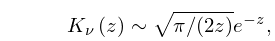
12: 10.25 Definitions

… ►In particular, the principal branch of $I_{\nu }\left(z\right)$ is defined in a similar way: it corresponds to the principal value of ${(\frac{1}{2}z)}^{\nu }$, is analytic in $ℂ\setminus (-\mathrm{\infty },0]$, and two-valued and discontinuous on the cut $\mathrm{ph}z=\pm \pi$. … ►

10.25.3 $$K_{\nu }\left(z\right)\sim \sqrt{\pi /(2z)}{\mathrm{e}}^{-z},$$

ⓘ

Defines:

$K_{\nu }\left(z\right)$: modified Bessel function of the second kind

Symbols:

$\sim$: asymptotic equality, $\pi$: the ratio of the circumference of a circle to its diameter, $\mathrm{e}$: base of natural logarithm, $z$: complex variable and $\nu$: complex parameter

Referenced by:

§10.25(ii), §10.25(iii), §10.30(ii)

Permalink:

http://dlmf.nist.gov/10.25.E3

Encodings:

pMML, png, TeX

See also:

Annotations for §10.25(ii), §10.25 and Ch.10

… ►It has a branch point at $z=0$ for all $\nu \in ℂ$. The principal branch corresponds to the principal value of the square root in (10.25.3), is analytic in $ℂ\setminus (-\mathrm{\infty },0]$, and two-valued and discontinuous on the cut $\mathrm{ph}z=\pm \pi$. …

13: 23.20 Mathematical Applications

… ►Points $P=(x,y)$ on the curve can be parametrized by $x=\mathrm{\wp }(z;g_2,g_3)$, $2y={\mathrm{\wp }}^{\prime }(z;g_2,g_3)$, where $g_2=-4a$ and $g_3=-4b$: in this case we write $P=P(z)$. The curve $C$ is made into an abelian group (Macdonald (1968, Chapter 5)) by defining the zero element $o=(0,1,0)$ as the point at infinity, the negative of $P=(x,y)$ by $-P=(x,-y)$, and generally $P_1+P_2+P_3=0$ on the curve iff the points $P_1$, $P_2$, $P_3$ are collinear. It follows from the addition formula (23.10.1) that the points $P_j=P(z_j)$, $j=1,2,3$, have zero sum iff $z_1+z_2+z_3\in 𝕃$, so that addition of points on the curve $C$ corresponds to addition of parameters $z_j$ on the torus $ℂ/𝕃$; see McKean and Moll (1999, §§2.11, 2.14). ►In terms of $(x,y)$ the addition law can be expressed $(x,y)+o=(x,y)$, $(x,y)+(x,-y)=o$; otherwise $(x_1,y_1)+(x_2,y_2)=(x_3,y_3)$, where … ►Let $T$ denote the set of points on $C$ that are of finite order (that is, those points $P$ for which there exists a positive integer $n$ with $nP=o$), and let $I,K$ be the sets of points with integer and rational coordinates, respectively. …

14: 4.23 Inverse Trigonometric Functions

… ►In (4.23.1) and (4.23.2) the integration paths may not pass through either of the points $t=\pm 1$. The function ${(1-t^2)}^{1/2}$ assumes its principal value when $t\in (-1,1)$; elsewhere on the integration paths the branch is determined by continuity. …$\mathrm{Arctan}z$ and $\mathrm{Arccot}z$ have branch points at $z=\pm \mathrm{i}$; the other four functions have branch points at $z=\pm 1$. … ►Care needs to be taken on the cuts, for example, if then $1/(x+\mathrm{i}0)=(1/x)-\mathrm{i}0$. … ►where $z=x+\mathrm{i}y$ and $\pm z\notin (1,\mathrm{\infty })$ in (4.23.34) and (4.23.35), and in (4.23.36). …

15: 1.10 Functions of a Complex Variable

… ►If $D=ℂ\setminus (-\mathrm{\infty },0]$ and $z=r{\mathrm{e}}^{\mathrm{i}\theta }$, then one branch is $\sqrt{r}{\mathrm{e}}^{\mathrm{i}\theta /2}$, the other branch is $-\sqrt{r}{\mathrm{e}}^{\mathrm{i}\theta /2}$, with in both cases. Similarly if $D=ℂ\setminus [0,\mathrm{\infty })$, then one branch is $\sqrt{r}{\mathrm{e}}^{\mathrm{i}\theta /2}$, the other branch is $-\sqrt{r}{\mathrm{e}}^{\mathrm{i}\theta /2}$, with in both cases. … ► … ►Alternatively, take $z_0$ to be any point in $D$ and set $F(z_0)={\mathrm{e}}^{\alpha \ln \left(1-z_0\right)}{\mathrm{e}}^{\beta \ln \left(1+z_0\right)}$ where the logarithms assume their principal values. (Thus if $z_0$ is in the interval $(-1,1)$, then the logarithms are real.) …

16: 36.5 Stokes Sets

§36.5 Stokes Sets

►

§36.5(i) Definitions

►Stokes sets are surfaces (codimension one) in $𝐱$ space, across which ${\mathrm{\Psi }}_K(𝐱;k)$ or ${\mathrm{\Psi }}^{(\mathrm{U})}(𝐱;k)$ acquires an exponentially-small asymptotic contribution (in $k$), associated with a complex critical point of ${\mathrm{\Phi }}_K$ or . …where $j$ denotes a real critical point (36.4.1) or (36.4.2), and $\mu$ denotes a critical point with complex $t$ or $s,t$, connected with $j$ by a steepest-descent path (that is, a path where $\mathrm{\Re }\mathrm{\Phi }=\mathrm{constant}$) in complex $t$ or $(s,t)$ space. … ►Red and blue numbers in each region correspond, respectively, to the numbers of real and complex critical points that contribute to the asymptotics of the canonical integral away from the bifurcation sets. …

17: 18.2 General Orthogonal Polynomials

… ►

Orthogonality on Countable Sets

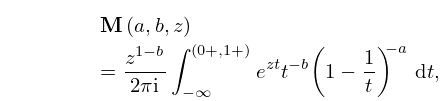
►Let $X$ be a finite set of distinct points on $ℝ$, or a countable infinite set of distinct points on $ℝ$, and $w_x$, $x\in X$, be a set of positive constants. …when $X$ is a finite set of $N+1$ distinct points. … ►If the orthogonality interval is $(-\mathrm{\infty },\mathrm{\infty })$ or $(0,\mathrm{\infty })$, then the role of $d/dx$ can be played by ${\delta }_x$, the central-difference operator in the imaginary direction (§18.1(i)). … ►If $d\mu \in 𝐌(a,b)$ then the interval $[b-a,b+a]$ is included in the support of $d\mu$, and outside $[b-a,b+a]$ the measure $d\mu$ only has discrete mass points $x_k$ such that $b\pm a$ are the only possible limit points of the sequence $\{x_k\}$, see Máté et al. (1991, Theorem 10). …

18: 13.4 Integral Representations

… ►The contour of integration starts and terminates at a point $\alpha$ on the real axis between $0$ and $1$. … ►

13.4.12 $$𝐌(a,c,z)=\frac{\mathrm{\Gamma }\left(b\right)}{2\pi \mathrm{i}}{z}^{1-b}{\int }_{-\mathrm{\infty }}^{(0+,1+)}{\mathrm{e}}^{zt}{t}^{-b}{}_2{}^{}𝐅_1^{}(a,b;c;1/t)dt,$$ $b\ne 0,-1,-2,\mathrm{\dots }$, .

ⓘ

Symbols:

$\mathrm{\Gamma }\left(z\right)$: gamma function, $𝐌(a,b,z)$: Olver’s confluent hypergeometric function, $\pi$: the ratio of the circumference of a circle to its diameter, $dx$: differential of $x$ , $\mathrm{e}$: base of natural logarithm, ${}_p{}^{}𝐅_q^{}(𝐚;𝐛;z)$ or ${}_p{}^{}𝐅_q^{}(\genfrac{}{}{0pt}{}{𝐚}{𝐛};z)$: scaled (or Olver’s) generalized hypergeometric function, $\mathrm{i}$: imaginary unit, $\int$: integral, $(a,b)$: open interval, $\mathrm{ph}$: phase and $z$: complex variable

Permalink:

http://dlmf.nist.gov/13.4.E12

Encodings:

pMML, png, TeX

See also:

Annotations for §13.4(ii), §13.4 and Ch.13

►At the point where the contour crosses the interval $(1,\mathrm{\infty })$, $t^{-b}$ and the ${}_2{}^{}𝐅_1^{}$ function assume their principal values; compare §§15.1 and 15.2(i). … ►

13.4.13 $$𝐌(a,b,z)=\frac{z^{1-b}}{2\pi \mathrm{i}}{\int }_{-\mathrm{\infty }}^{(0+,1+)}{\mathrm{e}}^{zt}{t}^{-b}{\left(1-\frac{1}{t}\right)}^{-a}dt,$$ .

ⓘ

Symbols:

$𝐌(a,b,z)$: Olver’s confluent hypergeometric function, $\pi$: the ratio of the circumference of a circle to its diameter, $dx$: differential of $x$ , $\mathrm{e}$: base of natural logarithm, $\mathrm{i}$: imaginary unit, $\int$: integral, $(a,b)$: open interval, $\mathrm{ph}$: phase and $z$: complex variable

Permalink:

http://dlmf.nist.gov/13.4.E13

Encodings:

pMML, png, TeX

See also:

Annotations for §13.4(ii), §13.4 and Ch.13

… ►At this point the fractional powers are determined by $\mathrm{ph}t=\pi$ and $\mathrm{ph}\left(1+t\right)=0$. …

19: 36.7 Zeros

… ►The zeros in Table 36.7.1 are points in the $𝐱=(x,y)$ plane, where $\mathrm{ph}{\mathrm{\Psi }}_2\left(𝐱\right)$ is undetermined. … ►Deep inside the bifurcation set, that is, inside the three-cusped astroid (36.4.10) and close to the part of the $z$-axis that is far from the origin, the zero contours form an array of rings close to the planes …The rings are almost circular (radii close to $(\Delta x)/9$ and varying by less than 1%), and almost flat (deviating from the planes $z_n$ by at most $(\Delta z)/36$). …Outside the bifurcation set (36.4.10), each rib is flanked by a series of zero lines in the form of curly “antelope horns” related to the “outside” zeros (36.7.2) of the cusp canonical integral. There are also three sets of zero lines in the plane $z=0$ related by $2\pi /3$ rotation; these are zeros of (36.2.20), whose asymptotic form in polar coordinates $(x=r\cos \theta ,y=r\sin \theta )$ is given by …

20: 25.12 Polylogarithms

… ►

25.12.2 $${\mathrm{Li}}_2\left(z\right)=-{\int }_0^z{t}^{-1}\ln \left(1-t\right)dt,$$ $z\in ℂ\setminus (1,\mathrm{\infty })$.

ⓘ

Symbols:

$ℂ$: complex plane, $dx$: differential of $x$ , ${\mathrm{Li}}_2\left(z\right)$: dilogarithm, $\in$: element of, $\int$: integral, $\ln z$: principal branch of logarithm function, $(a,b)$: open interval, $\setminus$: set subtraction, $x$: real variable and $z$: complex variable

Keywords:

definite integral, integral representation

Source:

Maximon (2003, (2.1), p. 2807)

A&S Ref:

27.7.1 (is a modified form with $z=1-x$)

Referenced by:

§25.12(i)

Permalink:

http://dlmf.nist.gov/25.12.E2

Encodings:

pMML, png, TeX

See also:

Annotations for §25.12(i), §25.12 and Ch.25

… ►In the complex plane ${\mathrm{Li}}_2\left(z\right)$ has a branch point at $z=1$. The principal branch has a cut along the interval $[1,\mathrm{\infty })$ and agrees with (25.12.1) when $|z|\le 1$; see also §4.2(i). … ►

25.12.3 $${\mathrm{Li}}_2\left(z\right)+{\mathrm{Li}}_2\left(\frac{z}{z-1}\right)=-\frac{1}{2}{(\ln \left(1-z\right))}^2,$$ $z\in ℂ\setminus [1,\mathrm{\infty })$.

ⓘ

Symbols:

$[a,b)$: half-closed interval, $ℂ$: complex plane, ${\mathrm{Li}}_2\left(z\right)$: dilogarithm, $\in$: element of, $\ln z$: principal branch of logarithm function, $\setminus$: set subtraction, $x$: real variable and $z$: complex variable

Keywords:

connection formula

Source:

Maximon (2003, (3.4), p. 2808)

A&S Ref:

27.7.5 (is a modified form with $z=1-x$)

Permalink:

http://dlmf.nist.gov/25.12.E3

Encodings:

pMML, png, TeX

See also:

Annotations for §25.12(i), §25.12 and Ch.25

… ►Sometimes the factor $1/\mathrm{\Gamma }\left(s+1\right)$ is omitted. …