on intervals
(0.002 seconds)
21—30 of 237 matching pages
21: About Color Map
…
►Mathematically, we scale the height to lying in the interval
and the components are computed as follows
…
►Specifically, by scaling the phase angle in to in the interval
, the hue (in degrees) is computed as
…
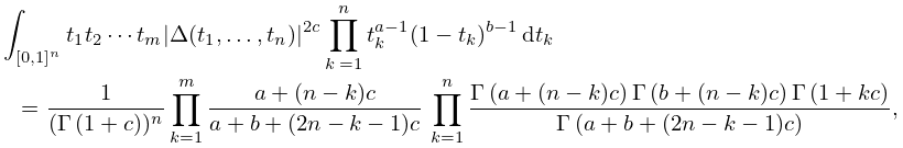
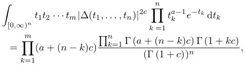
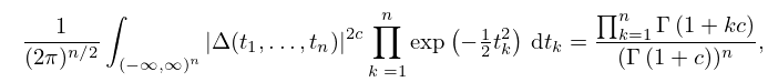
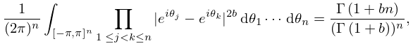
22: 5.14 Multidimensional Integrals
23: 18.2 General Orthogonal Polynomials
…
►
Orthogonality on Intervals
►Let be a finite or infinite open interval in . … ►Assume that the interval is bounded. … ►The Nevai class
… ►For OP’s on with weight function and orthogonality relation (18.2.5_5) assume that and is non-decreasing in the interval . …24: 31.15 Stieltjes Polynomials
…
►then there are exactly
polynomials , each of which corresponds to each of the ways of distributing its zeros among
intervals
, .
…
►If the exponent and singularity parameters satisfy (31.15.5)–(31.15.6), then for every multi-index , where each is a nonnegative integer, there is a unique Stieltjes polynomial with zeros in the open interval
for each .
…
►
31.15.8
,
►
31.15.9
,
…
►
31.15.10
…
25: 18.3 Definitions
…
►
Table 18.3.1: Orthogonality properties for classical OP’s: intervals, weight functions, standardizations, leading coefficients, and parameter constraints.
…
►
►
►
…
►
| Name | Constraints | ||||||
|---|---|---|---|---|---|---|---|
| … | |||||||
Jacobi on Other Intervals
►For a finite system of Jacobi polynomials is orthogonal on with weight function . For and a finite system of Jacobi polynomials (called pseudo Jacobi polynomials or Routh–Romanovski polynomials) is orthogonal on with . …26: 23.1 Special Notation
…
►
►
…
| lattice in . | |
| … | |
| or | closed, or open, straight-line segment joining and , whether or not and are real. |
| … | |
| Cartesian product of groups and , that is, the set of all pairs of elements with group operation . | |
27: 8.13 Zeros
…
►The negative zero decreases monotonically in the interval
, and satisfies
…
►
(a)
►
(b)
…
►
two zeros in each of the intervals when ;
two zeros in each of the intervals when ;
28: 3.11 Approximation Techniques
…
►Let be continuous on a closed interval
.
…
►For general intervals
we rescale:
…
►Let be continuous on a closed interval
and be a continuous nonvanishing function on : is called a weight function.
…of type
to on minimizes the maximum value of on , where
…
►Two are endpoints: and ; the other points and are control points.
…
29: 14.21 Definitions and Basic Properties
…
►When is complex , , and are defined by (14.3.6)–(14.3.10) with replaced by : the principal branches are obtained by taking the principal values of all the multivalued functions appearing in these representations when , and by continuity elsewhere in the -plane with a cut along the interval
; compare §4.2(i).
The principal branches of and are real when , and .
…
►Many of the properties stated in preceding sections extend immediately from the -interval
to the cut -plane .
…
