on a point set
(0.010 seconds)
21—30 of 113 matching pages
21: Mathematical Introduction
…
►The mathematical content of the NIST Handbook of Mathematical Functions has been produced over a ten-year period.
…
►First, the editors instituted a validation process for the whole technical content of each chapter.
…
►Secondly, as described in the Preface, a Web version (the NIST DLMF) is also available.
…
►These include, for example, multivalued functions of complex variables, for which new definitions of branch points and principal values are supplied (§§1.10(vi), 4.2(i)); the Dirac delta (or delta function), which is introduced in a more readily comprehensible way for mathematicians (§1.17); numerically satisfactory solutions of differential and difference equations (§§2.7(iv), 2.9(i)); and numerical analysis for complex variables (Chapter 3).
…
►Special functions with a complex variable are depicted as colored 3D surfaces in a similar way to functions of two real variables, but with the vertical height corresponding to the modulus (absolute value) of the function.
…
22: 18.38 Mathematical Applications
…
►The terminology DVR arises as an otherwise continuous variable, such as the co-ordinate , is replaced by its values at a finite set of zeros of appropriate OP’s resulting in expansions using functions localized at these points.
…
23: 33.23 Methods of Computation
…
►Inside the turning points, that is, when , there can be a loss of precision by a factor of approximately .
…
►WKBJ approximations (§2.7(iii)) for are presented in Hull and Breit (1959) and Seaton and Peach (1962: in Eq.
(12) should be ).
A set of consistent second-order WKBJ formulas is given by Burgess (1963: in Eq.
…
►Hull and Breit (1959) and Barnett (1981b) give WKBJ approximations for and in the region inside the turning point: .
24: 29.2 Differential Equations
…
►This equation has regular singularities at the points
, where , and , are the complete elliptic integrals of the first kind with moduli , , respectively; see §19.2(ii).
In general, at each singularity each solution of (29.2.1) has a branch point (§2.7(i)).
…
►
…
►
29.2.8
…
►Equation (29.2.10) is a special case of Heun’s equation (31.2.1).
…
25: Bibliography M
…
►
…
26: 3.4 Differentiation
…
►With the choice (which is crucial when is large because of numerical cancellation) the integrand equals at the dominant points
, and in combination with the factor in front of the integral sign this gives a rough approximation to .
…
27: 28.33 Physical Applications
…
►As runs from to , with and fixed, the point
moves from to along the ray given by the part of the line that lies in the first quadrant of the -plane.
…
28: 1.16 Distributions
…
►The closure of the set of points where is called the support of .
If the support of is a compact set (§1.9(vii)), then is called a function of compact
support.
…
►A sequence of test functions converges to a test function if the support of every is contained in a fixed compact set
and as the sequence converges uniformly on to for .
…
►If is a multi-index and , then we write and .
…
►Here ranges over a finite set of multi-indices, is a multivariate polynomial, and is a partial differential operator.
…
29: 1.4 Calculus of One Variable
…
►If is continuous at each point
, then is continuous on the interval
and we write .
…
►where the supremum is over all sets of points
in the closure of , that is, with added when they are finite.
…
