of%20the%20pth%20order
(0.002 seconds)
21—30 of 328 matching pages
21: 10.3 Graphics
…
►
►
 ►
►
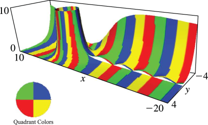
Figure 10.3.14:
, , .
…
Magnify
3D
Help
…
►
►
 ►
►
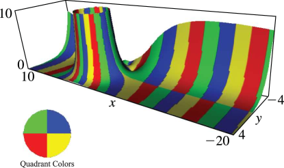
Figure 10.3.16:
, , .
…
Magnify
3D
Help
►
§10.3(i) Real Order and Variable
… ►§10.3(ii) Real Order, Complex Variable
… ►
§10.3(iii) Imaginary Order, Real Variable
…22: Foreword
…
►November 20, 2009
…
23: 13.30 Tables
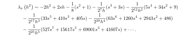
24: 28.16 Asymptotic Expansions for Large
…
►
28.16.1
…
25: 7.24 Approximations
…
►
•
…
►
•
…
Cody (1969) provides minimax rational approximations for and . The maximum relative precision is about 20S.
Cody et al. (1970) gives minimax rational approximations to Dawson’s integral (maximum relative precision 20S–22S).
26: 25.3 Graphics
27: 25.12 Polylogarithms
…
►
► ►
►
Figure 25.12.1: Dilogarithm function ,
Magnify
►
►
 ►
►
Figure 25.12.2: Absolute value of the dilogarithm function , , .
…
Magnify
3D
Help
…
►
28: 3.4 Differentiation
29: 9.18 Tables
…
►
•
…
►
•
…
►
•
►
•
►
•
…
Miller (1946) tabulates , for , for ; , for ; , for ; , , , (respectively , , , ) for . Precision is generally 8D; slightly less for some of the auxiliary functions. Extracts from these tables are included in Abramowitz and Stegun (1964, Chapter 10), together with some auxiliary functions for large arguments.
Zhang and Jin (1996, p. 337) tabulates , , , for to 8S and for to 9D.
Sherry (1959) tabulates , , , , ; 20S.
Zhang and Jin (1996, p. 339) tabulates , , , , , , , , ; 8D.
