normal values
(0.001 seconds)
11—20 of 58 matching pages
11: 23.23 Tables
…
►2 in Abramowitz and Stegun (1964) gives values of , , and to 7 or 8D in the rectangular and rhombic cases, normalized so that and (rectangular case), or and (rhombic case), for = 1.
…
12: 29.6 Fourier Series
…
►This solution can be constructed from (29.6.4) by backward recursion, starting with and an arbitrary nonzero value of , followed by normalization via (29.6.5) and (29.6.6).
…
13: 28.14 Fourier Series
…
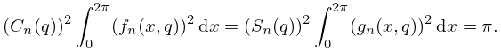
►and the normalization relation
►
28.14.5
…
►Ambiguities in sign are resolved by (28.14.9) when , and by continuity for other values of .
…
14: 28.5 Second Solutions ,
…
►The factors and in (28.5.1) and (28.5.2) are normalized so that
►
28.5.5
…
►(Other normalizations for and can be found in the literature, but most formulas—including connection formulas—are unaffected since and are invariant.)
…
►
…
15: 10.74 Methods of Computation
…
►In the case of , the need for initial values can be avoided by application of Olver’s algorithm (§3.6(v)) in conjunction with Equation (10.12.4) used as a normalizing condition, or in the case of noninteger orders, (10.23.15).
…
16: 6.18 Methods of Computation
…
►
, , and can be computed by Miller’s algorithm (§3.6(iii)), starting with initial values
, say, where is an arbitrary large integer, and normalizing via .
…
17: 33.9 Expansions in Series of Bessel Functions
…
►The series (33.9.1) converges for all finite values of and .
…
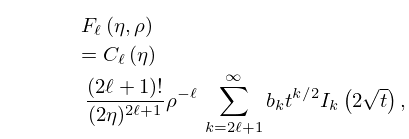
►
33.9.3
,
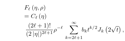
►
33.9.4
.
…
►The series (33.9.3) and (33.9.4) converge for all finite positive values of and .
…
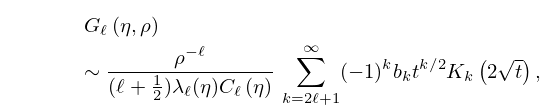
►
33.9.6
…
18: 14.30 Spherical and Spheroidal Harmonics
…
►
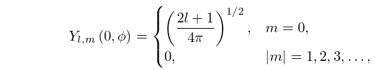
Special Values
►
14.30.4
…
►has solutions , which are everywhere one-valued and continuous.
►In the quantization of angular momentum the spherical harmonics are normalized solutions of the eigenvalue equations
…
19: 33.13 Complex Variable and Parameters
…
►The functions , , and may be extended to noninteger values of by generalizing , and supplementing (33.6.5) by a formula derived from (33.2.8) with expanded via (13.2.42).
►These functions may also be continued analytically to complex values of , , and .
…
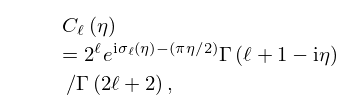
►
33.13.1
…
►
33.13.2
…
