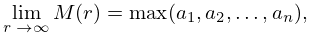
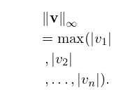
maximum

SearchAdvancedHelp

(0.001 seconds)

31—40 of 75 matching pages

31: Bibliography C

… ►

Determination of $\nu$-zeros of Hankel functions. Comput. Phys. Comm. 32 (3), pp. 333–339.

ⓘ

Notes:

Double-precision Fortran, maximum accuracy 7S.

External Links:

ISSN 0010-4655, Document, Code

Referenced by:

1st item.

Encodings:

BibTeX

… ►

Algorithm 352: Characteristic values and associated solutions of Mathieu’s differential equation. Comm. ACM 12 (7), pp. 399–407.

ⓘ

Notes:

Includes double-precision Fortran program, maximum accuracy 13D.

External Links:

ISSN 0001-0782, Document

Referenced by:

§28.36(ii), §28.36(iii).

Encodings:

BibTeX

… ►

Numerical evaluation of the Fermi-Dirac integrals. The Astrophysical Journal Supplement Series 71, pp. 677–699.

ⓘ

Notes:

Double-precision Fortran, maximum precision 12D.

External Links:

ISSN 0067-0049, Document, Code

Referenced by:

§25.12(iii), §25.18(i), 3rd item, 3rd item.

Encodings:

BibTeX

… ►

Algorithm 597: Sequence of modified Bessel functions of the first kind. ACM Trans. Math. Software 9 (2), pp. 242–245.

ⓘ

Notes:

Double-precision Fortran, maximum accuracy 24S.

External Links:

ISSN 0098-3500, Document, GAMS (module 597; package TOMS), ZentralBlatt

Referenced by:

5th item.

Encodings:

BibTeX

… ►

Algorithm AS 24: From normal integral to deviate. Appl. Statist. 18 (3), pp. 290–293.

ⓘ

Notes:

Includes Fortran program, maximum accuracy 12D.

External Links:

FullText

Referenced by:

§7.25(ii).

Encodings:

BibTeX

…

32: Bibliography H

… ►

Algorithm 55: Complete elliptic integral of the first kind. Comm. ACM 4 (4), pp. 180.

ⓘ

Notes:

Includes Algol program, maximum accuracy 8D. For certification see same journal 6 (1966), pp. 166–167

External Links:

ISSN 0001-0782, Document

Referenced by:

§19.39(ii).

Encodings:

BibTeX

►

Algorithm 56: Complete elliptic integral of the second kind. Comm. ACM 4 (4), pp. 180–181.

ⓘ

Notes:

Includes Algol program, maximum accuracy 8D. For certification see same journal 9 (1966), p. 12

External Links:

ISSN 0001-0782, Document

Referenced by:

§19.39(ii).

Encodings:

BibTeX

… ►

Algorithm 395: Student’s t-distribution. Comm. ACM 13 (10), pp. 617–619.

ⓘ

Notes:

Includes Algol program, maximum accuracy 11S. For Remarks see ACM Trans. Math. Software 5(1979) and 7(1981)

External Links:

ISSN 0001-0782, Document, Remark 1, Remark 2

Referenced by:

§8.28(iv).

Encodings:

BibTeX

… ►

Algorithm AS66: The normal integral. Appl. Statist. 22 (3), pp. 424–427.

ⓘ

Notes:

Double-precision Fortran, maximum accuracy 12D.

External Links:

FullText, Code

Referenced by:

5th item.

Encodings:

BibTeX

…

33: Bibliography S

… ►

Parabolic cylinder functions of integer and half-integer orders for nonnegative arguments. Comput. Phys. Comm. 115 (1), pp. 69–86.

ⓘ

Notes:

Double-precision Fortran, minimum accuracy 14S, maximum accuracy 18D.

External Links:

ISSN 0010-4655, Document, Code, MathReview, ZentralBlatt

Referenced by:

3rd item.

Encodings:

BibTeX

… ►

Algorithm 723: Fresnel integrals. ACM Trans. Math. Software 19 (4), pp. 452–456.

ⓘ

Notes:

Single- and double-precision Fortran, maximum accuracy 16D. For remarks see same journal v. 22 (1996), p. 498-500 and v. 26 (2000), p. 617

External Links:

ISSN 0098-3500, Document, GAMS (module 723; package TOMS), ZentralBlatt

Referenced by:

3rd item, 1st item.

Encodings:

BibTeX

… ►

On numerical Bessel transformation. Comput. Phys. Comm. 16 (3), pp. 383–387.

ⓘ

Notes:

Single-precision Fortran, maximum accuracy 15D.

External Links:

ISSN 0010-4655, Document, Code

Referenced by:

8th item.

Encodings:

BibTeX

… ►

Automatic computing methods for special functions. I. J. Res. Nat. Bur. Standards Sect. B 74B, pp. 211–224.

ⓘ

Notes:

Includes Fortran code, maximum accuracy 18S.

External Links:

MathReview (Bernard H. Rosman), ZentralBlatt

Referenced by:

§7.25(ii).

Encodings:

BibTeX

… ►

Root-rational-fraction package for exact calculation of vector-coupling coefficients. Comput. Phys. Comm. 21 (2), pp. 195–205.

ⓘ

Notes:

Double-precision Fortran, maximum accuracy 16D

External Links:

Document, Code

Referenced by:

10th item.

Encodings:

BibTeX

…

34: 28.22 Connection Formulas

… ►Here ${\mathrm{me}}_{\nu }(0,h^2)$ $(\ne 0)$ is given by (28.14.1) with $z=0$, and ${\mathrm{M}}_{\nu }^{(1)}(0,h)$ is given by (28.24.1) with $j=1$, $z=0$, and $n$ chosen so that $|c_{2n}^{\nu }(h^2)|=\max (|c_{2\mathrm{\ell }}^{\nu }(h^2)|)$, where the maximum is taken over all integers $\mathrm{\ell }$. …

35: Bibliography B

… ►

A program for computing the Fermi-Dirac functions. Comput. Phys. Comm. 21 (3), pp. 315–322.

ⓘ

Notes:

Double-precision Fortran, maximum accuracy 10D.

External Links:

Document, Code

Referenced by:

2nd item.

Encodings:

BibTeX

►

A program for computing the Riemann zeta function for complex argument. Comput. Phys. Comm. 20 (3), pp. 441–445.

ⓘ

Notes:

Double-precision Fortran, maximum accuracy 10S.

External Links:

Document, Code, ZentralBlatt

Referenced by:

1st item.

Encodings:

BibTeX

… ►

COULFG: Coulomb and Bessel functions and their derivatives, for real arguments, by Steed’s method. Comput. Phys. Comm. 27, pp. 147–166.

ⓘ

Notes:

Double-precision Fortran code for positive energies. Maximum accuracy: 31S.

External Links:

Document, Code

Referenced by:

2nd item, 2nd item.

Encodings:

BibTeX

… ►

Portable vectorized software for Bessel function evaluation. ACM Trans. Math. Software 18 (4), pp. 456–469.

ⓘ

Notes:

Single- and double-precision Fortran, maximum accuracy 17D. For corrigendum see same journal 19(1993), p. 131

External Links:

ISSN 0098-3500, Document, GAMS (package VFNLIB), ZentralBlatt

Referenced by:

2nd item.

Encodings:

BibTeX

… ►

Associated Legendre polynomials, ordinary and modified spherical harmonics. Comput. Phys. Comm. 5 (5), pp. 390–394.

ⓘ

Notes:

Single-precision Fortran, maximum accuracy 16S

External Links:

Document, Code

Referenced by:

2nd item.

Encodings:

BibTeX

…

36: Bibliography N

… ►

Algorithm 707: CONHYP: A numerical evaluator of the confluent hypergeometric function for complex arguments of large magnitudes. ACM Trans. Math. Software 18 (3), pp. 345–349.

ⓘ

Notes:

Double-precision Fortran, minimum accuracy 9S, maximum accuracy 13S.

External Links:

ISSN 0098-3500, Document, GAMS (module 707; package TOMS), ZentralBlatt

Referenced by:

1st item.

Encodings:

BibTeX

►

Numerical evaluation of the confluent hypergeometric function for complex arguments of large magnitudes. J. Comput. Appl. Math. 39 (2), pp. 193–200.

ⓘ

Notes:

Extended-precision Fortran evaluator, minimum accuracy 9S, maximum accuracy 13S.

External Links:

ISSN 0377-0427, Document, MathReview Entry, ZentralBlatt

Referenced by:

§13.32(iii).

Encodings:

BibTeX

…

37: 10.17 Asymptotic Expansions for Large Argument

… ►Then the remainder associated with the sum ${\sum }_{k=0}^{\mathrm{\ell }-1}{(-1)}^k{a}_{2k}(\nu )z^{-2k}$ does not exceed the first neglected term in absolute value and has the same sign provided that $\mathrm{\ell }\ge \max (\frac{1}{2}\nu -\frac{1}{4},1)$. Similarly for ${\sum }_{k=0}^{\mathrm{\ell }-1}{(-1)}^k{a}_{2k+1}(\nu )z^{-2k-1}$, provided that $\mathrm{\ell }\ge \max (\frac{1}{2}\nu -\frac{3}{4},1)$. … ►If these expansions are terminated when $k=\mathrm{\ell }-1$, then the remainder term is bounded in absolute value by the first neglected term, provided that $\mathrm{\ell }\ge \max (\nu -\frac{1}{2},1)$. …

38: 13.23 Integrals

… ►

13.23.11 $${\int }_0^{\mathrm{\infty }}{\mathrm{e}}^{\frac{1}{2}t}{t}^{\frac{1}{2}(\nu -1)-\mu }{W}_{\kappa ,\mu }\left(t\right)J_{\nu }\left(2\sqrt{xt}\right)dt=\frac{\mathrm{\Gamma }\left(\nu -2\mu +1\right)}{\mathrm{\Gamma }\left(\frac{1}{2}+\mu -\kappa \right)}{\mathrm{e}}^{\frac{1}{2}x}{x}^{\frac{1}{2}(\mu -\kappa -\frac{3}{2})}{W}_{\frac{1}{2}(\kappa +3\mu -\nu -\frac{1}{2}),\frac{1}{2}(\kappa -\mu +\nu +\frac{1}{2})}\left(x\right),$$ $x>0$, ,

ⓘ

Symbols:

$J_{\nu }\left(z\right)$: Bessel function of the first kind, $\mathrm{\Gamma }\left(z\right)$: gamma function, $W_{\kappa ,\mu }\left(z\right)$: Whittaker confluent hypergeometric function, $dx$: differential of $x$ , $\mathrm{e}$: base of natural logarithm, $\int$: integral, $\mathrm{\Re }$: real part and $x$: real variable

Permalink:

http://dlmf.nist.gov/13.23.E11

Encodings:

pMML, png, TeX

See also:

Annotations for §13.23(iii), §13.23 and Ch.13

►

13.23.12 $${\int }_0^{\mathrm{\infty }}{\mathrm{e}}^{-\frac{1}{2}t}{t}^{\frac{1}{2}(\nu -1)-\mu }{W}_{\kappa ,\mu }\left(t\right)J_{\nu }\left(2\sqrt{xt}\right)dt=\frac{\mathrm{\Gamma }\left(\nu -2\mu +1\right)}{\mathrm{\Gamma }\left(\frac{3}{2}-\mu -\kappa +\nu \right)}{\mathrm{e}}^{-\frac{1}{2}x}{x}^{\frac{1}{2}(\mu +\kappa -\frac{3}{2})}{M}_{\frac{1}{2}(\kappa -3\mu +\nu +\frac{1}{2}),\frac{1}{2}(\nu -\mu -\kappa +\frac{1}{2})}\left(x\right),$$ $x>0$, .

ⓘ

Symbols:

$J_{\nu }\left(z\right)$: Bessel function of the first kind, $\mathrm{\Gamma }\left(z\right)$: gamma function, $M_{\kappa ,\mu }\left(z\right)$: Whittaker confluent hypergeometric function, $W_{\kappa ,\mu }\left(z\right)$: Whittaker confluent hypergeometric function, $dx$: differential of $x$ , $\mathrm{e}$: base of natural logarithm, $\int$: integral, $\mathrm{\Re }$: real part and $x$: real variable

Permalink:

http://dlmf.nist.gov/13.23.E12

Encodings:

pMML, png, TeX

See also:

Annotations for §13.23(iii), §13.23 and Ch.13

… ►Then for $\mu$ in the half-plane $\mathrm{\Re }\mu \ge {\mu }_1>\max (-{\rho }_0,\mathrm{\Re }\kappa -\frac{1}{2})$ …

39: 1.2 Elementary Algebra

… ►

1.2.23 $$\underset{r\to \mathrm{\infty }}{lim}M(r)=\max (a_1,a_2,\mathrm{\dots },a_n),$$

ⓘ

Symbols:

$n$: nonnegative integer and $M(r)$: weighted mean

A&S Ref:

3.1.16

Permalink:

http://dlmf.nist.gov/1.2.E23

Encodings:

pMML, png, TeX

See also:

Annotations for §1.2(iv), §1.2 and Ch.1

… ►

1.2.48 $${\Vert 𝐯\Vert }_{\mathrm{\infty }}=\max (\left|v_1\right|,\left|v_2\right|,\mathrm{\dots },\left|v_n\right|).$$

ⓘ

Defines:

${\Vert 𝐯\Vert }_{\mathrm{\infty }}$: l-infinity norm

Symbols:

$n$: nonnegative integer, $𝐯$: column vector and $\left|x\right|$: absolute value of $x$

Permalink:

http://dlmf.nist.gov/1.2.E48

Encodings:

pMML, png, TeX

See also:

Annotations for §1.2(v), §1.2(v), §1.2 and Ch.1

… ►

1.2.67 $$\Vert 𝐀\Vert =\underset{𝐱\in {𝐄}_n\setminus \left\{𝟎\right\}}{\max }\frac{\Vert 𝐀𝐱\Vert }{\Vert 𝐱\Vert }=\underset{\Vert 𝐱\Vert =1}{\max }\Vert 𝐀𝐱\Vert .$$

ⓘ

Defines:

$\Vert 𝐀\Vert$: matrix norm

Symbols:

$\in$: element of, $\setminus$: set subtraction, $\Vert 𝐯\Vert$: vector norm ($l$²), ${𝐄}_n$: space of $n$-dimensional vectors, real or complex, $𝐀$: non-defective matrix and $𝟎$: $m\times m$ matrix of zeros

Permalink:

http://dlmf.nist.gov/1.2.E67

Encodings:

pMML, png, TeX

See also:

Annotations for §1.2(vi), §1.2(vi), §1.2 and Ch.1

…

40: 1.5 Calculus of Two or More Variables

… ► $f(x,y)$ has a local minimum (maximum) at $(a,b)$ if … ►as $\max ((x_{j+1}-x_j)+(y_{k+1}-y_k))\to 0$. …