little q-Jacobi polynomials

(0.004 seconds)

11—20 of 271 matching pages

11: 34.8 Approximations for Large Parameters

… ►

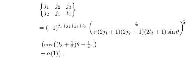
34.8.1

\begin{Bmatrix}j_{1}&j_{2}&j_{3}\\ j_{2}&j_{1}&l_{3}\end{Bmatrix}=(-1)^{j_{1}+j_{2}+j_{3}+l_{3}}\*\left(\frac{4}{% \pi(2j_{1}+1)(2j_{2}+1)(2l_{3}+1)\sin\theta}\right)^{\frac{1}{2}}\*\left(\cos% \left((l_{3}+\tfrac{1}{2})\theta-\tfrac{1}{4}\pi\right)+o\left(1\right)\right),

j_{1},j_{2},j_{3}\gg l_{3}\gg 1

ⓘ

Symbols:: $\pi$ : the ratio of the circumference of a circle to its diameter, $\cos\NVar{z}$ : cosine function, $o\left(\NVar{x}\right)$ : order less than, $\sin\NVar{z}$ : sine function, $\begin{Bmatrix}\NVar{j_{1}}&\NVar{j_{2}}&\NVar{j_{3}}\\ \NVar{l_{1}}&\NVar{l_{2}}&\NVar{l_{3}}\end{Bmatrix}$ : $\mathit{6j}$ symbol, $j,j_{r}$ : non-negative integers or non-negative integers plus one half. and $l,l_{r}$ : non-negative integers or non-negative integers plus one half.
Permalink:: http://dlmf.nist.gov/34.8.E1
Encodings:: pMML, png, TeX
See also:: Annotations for §34.8 and Ch.34

… ►and the symbol

o\left(1\right)

denotes a quantity that tends to zero as the parameters tend to infinity, as in §2.1(i). …

12: 2.10 Sums and Sequences

… ►As in §24.2, let

B_{n}

and

B_{n}\left(x\right)

denote the

n

th Bernoulli number and polynomial, respectively, and

\widetilde{B}_{n}\left(x\right)

the

n

th Bernoulli periodic function

B_{n}\left(x-\left\lfloor x\right\rfloor\right)

. … ►

(a)

On the strip $a\leq\Re z\leq n$ , $f(z)$ is analytic in its interior, $f^{(2m)}(z)$ is continuous on its closure, and $f(z)=o\left(e^{2\pi|\Im z|}\right)$ as $\Im z\to\pm\infty$ , uniformly with respect to $\Re z\in[a,n]$ .

… ►From §24.12(i), (24.2.2), and (24.4.27),

\widetilde{B}_{2m}\left(x\right)-B_{2m}

is of constant sign

(-1)^{m}

. … ►

Example

►Let

\alpha

be a constant in

(0,2\pi)

and

P_{n}

denote the Legendre polynomial of degree

n

. …

13: 33.10 Limiting Forms for Large $\rho$ or Large $\left|\eta\right|$

… ►

F_{\ell}\left(\eta,\rho\right)=\sin\left({\theta_{\ell}}\left(\eta,\rho\right)% \right)+o\left(1\right),

►

G_{\ell}\left(\eta,\rho\right)=\cos\left({\theta_{\ell}}\left(\eta,\rho\right)% \right)+o\left(1\right),

… ►

{\sigma_{0}}\left(\eta\right)=\eta(\ln\eta-1)+\tfrac{1}{4}\pi+o\left(1\right),

… ►

F_{0}\left(\eta,\rho\right)=(\pi\rho)^{\ifrac{1}{2}}J_{1}\left((-8\eta\rho)^{% \ifrac{1}{2}}\right)+o\left({\left|\eta\right|}^{-\ifrac{1}{4}}\right),

… ►

{\sigma_{0}}\left(\eta\right)=\eta(\ln\left(-\eta\right)-1)-\tfrac{1}{4}\pi+o% \left(1\right),

…

14: 18.28 Askey–Wilson Class

… ►

Duality

… ►

§18.28(v) Continuous $q$ -Ultraspherical Polynomials

… ►These polynomials are also called Rogers polynomials. ►

§18.28(vi) Continuous $q$ -Hermite Polynomials

… ►

From Askey–Wilson to Little $q$ -Jacobi

…

15: 2.1 Definitions and Elementary Properties

… ►

2.1.2

\displaystyle f(x)=o\left(\phi(x)\right)\Longleftrightarrow f(x)/\phi(x)\to 0.

ⓘ

Defines:: $o\left(\NVar{x}\right)$ : order less than
Permalink:: http://dlmf.nist.gov/2.1.E2
Encodings:: pMML, png, TeX
See also:: Annotations for §2.1(i), §2.1 and Ch.2

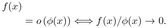
… ►The symbols

o

and

O

can be used generically. … ►

o\left(\phi\right)=O\left(\phi\right)

►

o\left(\phi\right)+o\left(\phi\right)=o\left(\phi\right)

… ►This result also holds with both

O

’s replaced by

o

’s. …

16: 28.29 Definitions and Basic Properties

… ►

\mu_{2m-1}-(2m-1)^{2}-\dfrac{N}{(4m)^{2}}=o\left(m^{-2}\right),

►

\mu_{2m}-(2m-1)^{2}-\dfrac{N}{(4m)^{2}}=o\left(m^{-2}\right),

►

\lambda_{2m-1}-(2m)^{2}-\dfrac{N}{(4m)^{2}}=o\left(m^{-2}\right),

… ►

\lambda_{2m}-\lambda_{2m-1}=o\left(\ifrac{1}{m^{k}}\right),

►

\mu_{2m}-\mu_{2m-1}=o\left(\ifrac{1}{m^{k}}\right);

…

17: 18.2 General Orthogonal Polynomials

§18.2 General Orthogonal Polynomials

… ►

Kernel Polynomials

… ►It is to be noted that, although formally correct, the results of (18.2.30) are of little utility for numerical work, as Hankel determinants are notoriously ill-conditioned. … ► … ►

Sheffer Polynomials

…

18: 18.40 Methods of Computation

… ►

§18.40(i) Computation of Polynomials

►Orthogonal polynomials can be computed from their explicit polynomial form by Horner’s scheme (§1.11(i)). … … ►There are many ways to implement these first two steps, noting that the expressions for

\alpha_{n}

and

\beta_{n}

of equation (18.2.30) are of little practical numerical value, see Gautschi (2004) and Golub and Meurant (2010). … ►The example chosen is inversion from the

\alpha_{n},\beta_{n}

for the weight function for the repulsive Coulomb–Pollaczek, RCP, polynomials of (18.39.50). …

19: 15.12 Asymptotic Approximations

… ►For the more general case in which

a^{2}=o\left(c\right)

and

b^{2}=o\left(c\right)

see Wagner (1990). … ►See also Dunster (1999) where the asymptotics of Jacobi polynomials is described; compare (15.9.1). …

20: 18.39 Applications in the Physical Sciences

… ►This material is employed below with little additional discussion. … ►The associated Coulomb–Laguerre polynomials are defined as … ►

§18.39(iv) Coulomb–Pollaczek Polynomials and J-Matrix Methods

… ►

The Coulomb–Pollaczek Polynomials

… ►

§18.39(v) Other Applications

…