limiting forms as trigonometric functions

(0.010 seconds)

21—30 of 39 matching pages

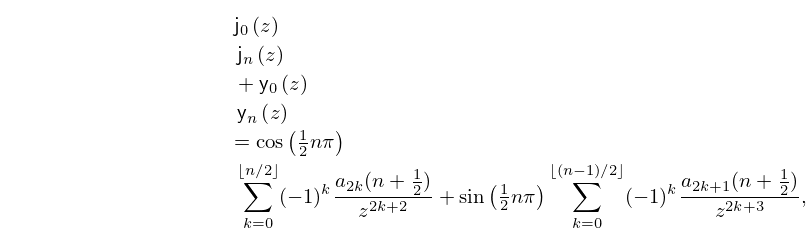
21: 10.50 Wronskians and Cross-Products

§10.50 Wronskians and Cross-Products

… ►

10.50.4

\mathsf{j}_{0}\left(z\right)\mathsf{j}_{n}\left(z\right)+\mathsf{y}_{0}\left(z% \right)\mathsf{y}_{n}\left(z\right)=\cos\left(\tfrac{1}{2}n\pi\right)\sum_{k=0% }^{\left\lfloor n/2\right\rfloor}(-1)^{k}\frac{a_{2k}(n+\tfrac{1}{2})}{z^{2k+2% }}+\sin\left(\tfrac{1}{2}n\pi\right)\sum_{k=0}^{\left\lfloor(n-1)/2\right% \rfloor}(-1)^{k}\frac{a_{2k+1}(n+\tfrac{1}{2})}{z^{2k+3}},

ⓘ

Symbols:: $\pi$ : the ratio of the circumference of a circle to its diameter, $\cos\NVar{z}$ : cosine function, $\left\lfloor\NVar{x}\right\rfloor$ : floor of $x$ , $\sin\NVar{z}$ : sine function, $\mathsf{j}_{\NVar{n}}\left(\NVar{z}\right)$ : spherical Bessel function of the first kind, $\mathsf{y}_{\NVar{n}}\left(\NVar{z}\right)$ : spherical Bessel function of the second kind, $n$ : integer, $k$ : nonnegative integer, $z$ : complex variable and $a_{k}(\nu)$ : polynomial coefficient
A&S Ref:: 10.1.33 (modified)
Referenced by:: §10.50, §10.50
Permalink:: http://dlmf.nist.gov/10.50.E4
Encodings:: pMML, png, TeX
See also:: Annotations for §10.50 and Ch.10

…

22: 8.11 Asymptotic Approximations and Expansions

§8.11 Asymptotic Approximations and Expansions

… ►where

\delta

denotes an arbitrary small positive constant. … ►For the function

e_{n}(z)

defined by (8.4.11), ►

8.11.13

\lim_{n\to\infty}\frac{e_{n}(nx)}{e^{nx}}=\begin{cases}0,&x>1,\\ \tfrac{1}{2},&x=1,\\ 1,&0\leq x<1.\end{cases}

ⓘ

Symbols:: $\mathrm{e}$ : base of natural logarithm, $x$ : real variable, $n$ : nonnegative integer and $e_{n}(z)$ : functions
A&S Ref:: 6.5.34 (Slightly modified)
Permalink:: http://dlmf.nist.gov/8.11.E13
Encodings:: pMML, png, TeX
See also:: Annotations for §8.11(v), §8.11 and Ch.8

… ►

23: 3.10 Continued Fractions

… ►However, other continued fractions with the same limit may converge in a much larger domain of the complex plane than the fraction given by (3.10.4) and (3.10.5). … ►A continued fraction of the form … ►A continued fraction of the form … ►For elementary functions, see §§ 4.9 and 4.35. … ►can be written in the form …

24: 7.14 Integrals

… ►

§7.14(i) Error Functions

►

Fourier Transform

… ►When

a=0

the limit is taken. ►

Laplace Transforms

… ►In a series of ten papers Hadži (1968, 1969, 1970, 1972, 1973, 1975a, 1975b, 1976a, 1976b, 1978) gives many integrals containing error functions and Fresnel integrals, also in combination with the hypergeometric function, confluent hypergeometric functions, and generalized hypergeometric functions.

25: 28.12 Definitions and Basic Properties

… ►

§28.12(ii) Eigenfunctions $\operatorname{me}_{\nu}\left(z,q\right)$

… ►However, these functions are not the limiting values of

\operatorname{me}_{\pm\nu}\left(z,q\right)

\nu\to n

(\neq 0)

. … ►Again, the limiting values of

\operatorname{ce}_{\nu}(z,q)

and

\operatorname{se}_{\nu}(z,q)

\nu\to n

(\neq 0)

are not the functions

\operatorname{ce}_{n}\left(z,q\right)

and

\operatorname{se}_{n}\left(z,q\right)

defined in §28.2(vi). …

26: 2.6 Distributional Methods

… ►This leads to integrals of the form … ►The distribution method outlined here can be extended readily to functions

f(t)

having an asymptotic expansion of the form … ►To define convolutions of distributions, we first introduce the space

K^{+}

of all distributions of the form

D^{n}f

, where

n

is a nonnegative integer,

f

is a locally integrable function on

\mathbb{R}

which vanishes on

(-\infty,0]

, and

D^{n}f

denotes the

n

th derivative of the distribution associated with

f

. …It is easily seen that

K^{+}

forms a commutative, associative linear algebra. … ►On inserting this identity into (2.6.54), we immediately encounter divergent integrals of the form …

27: 28.20 Definitions and Basic Properties

… ►with its algebraic form … ►

§28.20(iv) Radial Mathieu Functions ${\operatorname{Mc}^{(j)}_{n}}$ , ${\operatorname{Ms}^{(j)}_{n}}$

… ►

§28.20(vi) Wronskians

… ►

§28.20(vii) Shift of Variable

… ►When

\nu

is an integer the right-hand sides of (28.20.25) are replaced by the their limiting values. …

28: 1.18 Linear Second Order Differential Operators and Eigenfunction Expansions

… ►These are based on the Liouville normal form of (1.13.29). … ►The eigenfunctions form a complete orthogonal basis in

L^{2}\left(X\right)

, and we can take the basis as orthonormal: … ►Let

T

be the self adjoint extension of a formally self-adjoint differential operator

\mathcal{L}

of the form (1.18.28) on an unbounded interval

X\subset\mathbb{R}

, which we will take as

X=[0,+\infty)

, and assume that

q(x)\to 0

monotonically as

x\to\infty

, and that the eigenfunctions are non-vanishing but bounded in this same limit. … ► A boundary value for the end point

a

is a linear form

\mathcal{B}

\mathcal{D}({\mathcal{L}}^{*})

of the form …where

\alpha

and

\beta

are given functions on

X

, and where the limit has to exist for all

f

. …

29: 28.6 Expansions for Small $q$

… ►

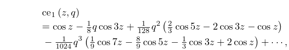
§28.6(ii) Functions $\operatorname{ce}_{n}$ and $\operatorname{se}_{n}$

►Leading terms of the power series for the normalized functions are: … ►

28.6.22

\operatorname{ce}_{1}\left(z,q\right)=\cos z-\tfrac{1}{8}q\cos 3z+\tfrac{1}{12% 8}q^{2}\left(\tfrac{2}{3}\cos 5z-2\cos 3z-\cos z\right)-\tfrac{1}{1024}q^{3}% \left(\tfrac{1}{9}\cos 7z-\tfrac{8}{9}\cos 5z-\tfrac{1}{3}\cos 3z+2\cos z% \right)+\cdots,

ⓘ

Symbols:: $\operatorname{ce}_{\NVar{n}}\left(\NVar{z},\NVar{q}\right)$ : Mathieu function, $\cos\NVar{z}$ : cosine function, $q=h^{2}$ : parameter and $z$ : complex variable
Permalink:: http://dlmf.nist.gov/28.6.E22
Encodings:: pMML, png, TeX
See also:: Annotations for §28.6(ii), §28.6 and Ch.28

… ►

28.6.26

\operatorname{ce}_{m}\left(z,q\right)=\cos mz-\frac{q}{4}\left(\frac{1}{m+1}% \cos(m+2)z-\frac{1}{m-1}\cos(m-2)z\right)+\frac{q^{2}}{32}\left(\frac{1}{(m+1)% (m+2)}\cos(m+4)z+\frac{1}{(m-1)(m-2)}\cos(m-4)z-\frac{2(m^{2}+1)}{(m^{2}-1)^{2% }}\cos mz\right)+\cdots.

ⓘ

Symbols:: $\operatorname{ce}_{\NVar{n}}\left(\NVar{z},\NVar{q}\right)$ : Mathieu function, $\cos\NVar{z}$ : cosine function, $m$ : integer, $q=h^{2}$ : parameter and $z$ : complex variable
A&S Ref:: 20.2.28 (in slightly different form)
Referenced by:: §28.6(ii), §28.6(ii), §28.6(ii), Erratum (V1.1.10) for Sections 28.6(i), 28.6(ii), 28.8(i), 28.8(ii)
Permalink:: http://dlmf.nist.gov/28.6.E26
Encodings:: pMML, png, TeX
See also:: Annotations for §28.6(ii), §28.6 and Ch.28

►For the corresponding expansions of

\operatorname{se}_{m}\left(z,q\right)

for

m=3,4,5,\dots

change

\cos

\sin

everywhere in (28.6.26). …

30: 3.3 Interpolation

… ►The final expression in (3.3.1) is the Barycentric form of the Lagrange interpolation formula. … … ►The

(n+1)

-point formula (3.3.4) can be written in the form … ►For example, for

k+1

coincident points the limiting form is given by

\left[z_{0},z_{0},\dots,z_{0}\right]f=f^{(k)}(z_{0})/k!

. … ►

§3.3(vi) Other Interpolation Methods

…