limiting forms as order tends to integers

SearchAdvancedHelp

(0.001 seconds)

21—30 of 929 matching pages

21: 13.2 Definitions and Basic Properties

… ►It can be regarded as the limiting form of the hypergeometric differential equation (§15.10(i)) that is obtained on replacing $z$ by $z/b$, letting $b\to \mathrm{\infty }$, and subsequently replacing the symbol $c$ by $b$. … ►Although $M(a,b,z)$ does not exist when $b=-n$, $n=0,1,2,\mathrm{\dots }$, many formulas containing $M(a,b,z)$ continue to apply in their limiting form. … ►When $m\in \mathbb{Z}$, … ►

§13.2(iii) Limiting Forms as $z\to 0$

… ►

§13.2(iv) Limiting Forms as $z\to \mathrm{\infty }$

…

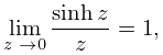
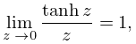
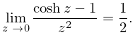
22: 4.31 Special Values and Limits

§4.31 Special Values and Limits

►

Table 4.31.1: Hyperbolic functions: values at multiples of $\frac{1}{2}\pi \mathrm{i}$.

► ►►

$z$	0	$\frac{1}{2}\pi \mathrm{i}$	$\pi \mathrm{i}$	$\frac{3}{2}\pi \mathrm{i}$	$\mathrm{\infty }$
…

►

►

4.31.1 $$\underset{z\to 0}{lim}\frac{\sinh z}{z}=1,$$

ⓘ

Symbols:

$\sinh z$: hyperbolic sine function and $z$: complex variable

Permalink:

http://dlmf.nist.gov/4.31.E1

Encodings:

pMML, png, TeX

See also:

Annotations for §4.31 and Ch.4

►

4.31.2 $$\underset{z\to 0}{lim}\frac{\tanh z}{z}=1,$$

ⓘ

Symbols:

$\tanh z$: hyperbolic tangent function and $z$: complex variable

Permalink:

http://dlmf.nist.gov/4.31.E2

Encodings:

pMML, png, TeX

See also:

Annotations for §4.31 and Ch.4

►

4.31.3 $$\underset{z\to 0}{lim}\frac{\cosh z-1}{z^2}=\frac{1}{2}.$$

ⓘ

Symbols:

$\cosh z$: hyperbolic cosine function and $z$: complex variable

Permalink:

http://dlmf.nist.gov/4.31.E3

Encodings:

pMML, png, TeX

See also:

Annotations for §4.31 and Ch.4

23: 33.21 Asymptotic Approximations for Large $|r|$

… ►

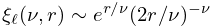
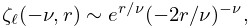
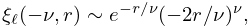
§33.21(i) Limiting Forms

►We indicate here how to obtain the limiting forms of $f(ϵ,\mathrm{\ell };r)$, $h(ϵ,\mathrm{\ell };r)$, $s(ϵ,\mathrm{\ell };r)$, and $c(ϵ,\mathrm{\ell };r)$ as $r\to \pm \mathrm{\infty }$, with $ϵ$ and $\mathrm{\ell }$ fixed, in the following cases: ►

When $r\to \pm \mathrm{\infty }$ with $ϵ>0$, Equations (33.16.4)–(33.16.7) are combined with (33.10.1).

►

When $r\to \pm \mathrm{\infty }$ with , Equations (33.16.10)–(33.16.13) are combined with

33.21.1

${\zeta }_{\mathrm{\ell }}(\nu ,r)\sim {\mathrm{e}}^{-r/\nu }{(2r/\nu )}^{\nu },$

${\xi }_{\mathrm{\ell }}(\nu ,r)\sim {\mathrm{e}}^{r/\nu }{(2r/\nu )}^{-\nu }$ , $r\to \mathrm{\infty }$,

ⓘ

Symbols:

$\sim$: asymptotic equality, $\mathrm{e}$: base of natural logarithm, $\mathrm{\ell }$: nonnegative integer, $r$: real variable, $\nu$: parameter, ${\zeta }_{\mathrm{\ell }}(\nu ,r)$: function and ${\xi }_{\mathrm{\ell }}(\nu ,r)$: function

Permalink:

http://dlmf.nist.gov/33.21.E1

Encodings:

pMML, pMML, png, png, TeX, TeX

See also:

Annotations for §33.21(i), §33.21 and Ch.33

33.21.2

${\zeta }_{\mathrm{\ell }}(-\nu ,r)\sim {\mathrm{e}}^{r/\nu }{(-2r/\nu )}^{-\nu },$

${\xi }_{\mathrm{\ell }}(-\nu ,r)\sim {\mathrm{e}}^{-r/\nu }{(-2r/\nu )}^{\nu },$ $r\to -\mathrm{\infty }$.

ⓘ

Symbols:

$\sim$: asymptotic equality, $\mathrm{e}$: base of natural logarithm, $\mathrm{\ell }$: nonnegative integer, $r$: real variable, $\nu$: parameter, ${\zeta }_{\mathrm{\ell }}(\nu ,r)$: function and ${\xi }_{\mathrm{\ell }}(\nu ,r)$: function

Permalink:

http://dlmf.nist.gov/33.21.E2

Encodings:

pMML, pMML, png, png, TeX, TeX

See also:

Annotations for §33.21(i), §33.21 and Ch.33

Corresponding approximations for $s(ϵ,\mathrm{\ell };r)$ and $c(ϵ,\mathrm{\ell };r)$ as $r\to \mathrm{\infty }$ can be obtained via (33.16.17), and as $r\to -\mathrm{\infty }$ via (33.16.18).

►

When $r\to \pm \mathrm{\infty }$ with $ϵ=0$, combine (33.20.1), (33.20.2) with §§10.7(ii), 10.30(ii).

…

24: 10.7 Limiting Forms

§10.7 Limiting Forms

►

§10.7(i) $z\to 0$

►When $\nu$ is fixed and $z\to 0$, … ►

§10.7(ii) $z\to \mathrm{\infty }$

►When $\nu$ is fixed and $z\to \mathrm{\infty }$, …

25: 22.5 Special Values

… ►Table 22.5.1 gives the value of each of the 12 Jacobian elliptic functions, together with its $z$-derivative (or at a pole, the residue), for values of $z$ that are integer multiples of $K$, $\mathrm{i}{K}^{\prime }$. … ►

§22.5(ii) Limiting Values of $k$

►If $k\to 0+$, then $K\to \pi /2$ and $K^{\prime }\to \mathrm{\infty }$; if $k\to 1-$, then $K\to \mathrm{\infty }$ and $K^{\prime }\to \pi /2$. … ►Expansions for $K,K^{\prime }$ as $k\to 0$ or $1$ are given in §§19.5, 19.12. … ►

26: 26.9 Integer Partitions: Restricted Number and Part Size

§26.9 Integer Partitions: Restricted Number and Part Size

►

§26.9(i) Definitions

… ►It follows that $p_k\left(n\right)$ also equals the number of partitions of $n$ into parts that are less than or equal to $k$. … ►Equations (26.9.2)–(26.9.3) are examples of closed forms that can be computed explicitly for any positive integer $k$. … ►

§26.9(iv) Limiting Form

…

27: Mathematical Introduction

… ►Other examples are: (a) the notation for the Ferrers functions—also known as associated Legendre functions on the cut—for which existing notations can easily be confused with those for other associated Legendre functions (§14.1); (b) the spherical Bessel functions for which existing notations are unsymmetric and inelegant (§§10.47(i) and 10.47(ii)); and (c) elliptic integrals for which both Legendre’s forms and the more recent symmetric forms are treated fully (Chapter 19). … ►In these cases the phase colors that correspond to the 1st, 2nd, 3rd, and 4th quadrants are arranged in alphabetical order: blue, green, red, and yellow, respectively, and a “Quadrant Colors” icon appears alongside the figure. … ►The purpose of these sections is simply to illustrate the importance of the functions in other disciplines; no attempt is made to provide exhaustive coverage. … ►For equations or other technical information that appeared previously in AMS 55, the DLMF usually includes the corresponding AMS 55 equation number, or other form of reference, together with corrections, if needed. … ►I pay tribute to my friend and predecessor Milton Abramowitz. …

28: 20.13 Physical Applications

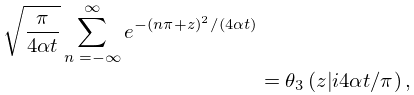
… ►For $\tau =\mathrm{i}t$, with $\alpha ,t,z$ real, (20.13.1) takes the form of a real-time $t$ diffusion equation … ►

20.13.4 $$\sqrt{\frac{\pi }{4\alpha t}}\sum _{n=-\mathrm{\infty }}^{\mathrm{\infty }}{\mathrm{e}}^{-{(n\pi +z)}^2/(4\alpha t)}={\theta }_3\left(z\right|\mathrm{i}4\alpha t/\pi ),$$

ⓘ

Symbols:

${\theta }_j\left(z\right|\tau )$: theta function, $\pi$: the ratio of the circumference of a circle to its diameter, $\mathrm{e}$: base of natural logarithm, $\mathrm{i}$: imaginary unit, $n$: integer, $t$: time, $\alpha$: real parameter and $z$: real variable

Permalink:

http://dlmf.nist.gov/20.13.E4

Encodings:

pMML, png, TeX

See also:

Annotations for §20.13 and Ch.20

… ►Theta-function solutions to the heat diffusion equation with simple boundary conditions are discussed in Lawden (1989, pp. 1–3), and with more general boundary conditions in Körner (1989, pp. 274–281). ►In the singular limit $\mathrm{\Im }\tau \to 0+$, the functions ${\theta }_j\left(z\right|\tau )$, $j=1,2,3,4$, become integral kernels of Feynman path integrals (distribution-valued Green’s functions); see Schulman (1981, pp. 194–195). This allows analytic time propagation of quantum wave-packets in a box, or on a ring, as closed-form solutions of the time-dependent Schrödinger equation.

29: 33.23 Methods of Computation

… ►The methods used for computing the Coulomb functions described below are similar to those in §13.29. … ►The power-series expansions of §§33.6 and 33.19 converge for all finite values of the radii $\rho$ and $r$, respectively, and may be used to compute the regular and irregular solutions. … ►In a similar manner to §33.23(iii) the recurrence relations of §§33.4 or 33.17 can be used for a range of values of the integer $\mathrm{\ell }$, provided that the recurrence is carried out in a stable direction (§3.6). … ►Curtis (1964a, §10) describes the use of series, radial integration, and other methods to generate the tables listed in §33.24. … ►A set of consistent second-order WKBJ formulas is given by Burgess (1963: in Eq. …

30: 11.9 Lommel Functions

… ►The inhomogeneous Bessel differential equation … ►the right-hand side being replaced by its limiting form when $\mu \pm \nu$ is an odd negative integer. … ►If either of $\mu \pm \nu$ equals an odd positive integer, then the right-hand side of (11.9.9) terminates and represents $S_{\mu ,\nu }\left(z\right)$ exactly. ►For uniform asymptotic expansions, for large $\nu$ and fixed $\mu =-1,0,1,2,\mathrm{\dots }$, of solutions of the inhomogeneous modified Bessel differential equation that corresponds to (11.9.1) see Olver (1997b, pp. 388–390). … …