lattice%20points

SearchAdvancedHelp

(0.001 seconds)

11—20 of 250 matching pages

11: 23.10 Addition Theorems and Other Identities

… ►

23.10.4 $$\sigma \left(u+v\right)\sigma \left(u-v\right)\sigma \left(x+y\right)\sigma \left(x-y\right)+\sigma \left(v+x\right)\sigma \left(v-x\right)\sigma \left(u+y\right)\sigma \left(u-y\right)+\sigma \left(x+u\right)\sigma \left(x-u\right)\sigma \left(v+y\right)\sigma \left(v-y\right)=0.$$

ⓘ

Symbols:

$\sigma \left(z\right)$ (= $\sigma \left(z|𝕃\right)$ = $\sigma (z;g_2,g_3)$): Weierstrass sigma function, $𝕃$: lattice, $x$: real part of $z$ and $y$: imaginary part of $z$

Permalink:

http://dlmf.nist.gov/23.10.E4

Encodings:

pMML, png, TeX

See also:

Annotations for §23.10(i), §23.10 and Ch.23

►For further addition-type identities for the $\sigma$-function see Lawden (1989, §6.4). … ►

23.10.8 $$(\mathrm{\wp }\left(2z\right)-e_1)\mathrm{\wp }_{}^{\prime }{}_{}{}^2(z)={\left({(\mathrm{\wp }\left(z\right)-e_1)}^2-(e_1-e_2)(e_1-e_3)\right)}^2.$$

ⓘ

Symbols:

$\mathrm{\wp }\left(z\right)$ (= $\mathrm{\wp }\left(z|𝕃\right)$ = $\mathrm{\wp }(z;g_2,g_3)$): Weierstrass $\mathrm{\wp }$-function, $e_j$: Weierstrass lattice roots, $𝕃$: lattice and $z$: complex

Referenced by:

§23.10(ii), §23.10(ii)

Permalink:

http://dlmf.nist.gov/23.10.E8

Encodings:

pMML, png, TeX

See also:

Annotations for §23.10(ii), §23.10 and Ch.23

►(23.10.8) continues to hold when $e_1$, $e_2$, $e_3$ are permuted cyclically. … ►Also, when $𝕃$ is replaced by $c𝕃$ the lattice invariants $g_2$ and $g_3$ are divided by $c^4$ and $c^6$, respectively. …

12: 20.2 Definitions and Periodic Properties

… ►The four points $(0,\pi ,\pi +\tau \pi ,\tau \pi )$ are the vertices of the fundamental parallelogram in the $z$-plane; see Figure 20.2.1. The points ►

20.2.5 $$z_{m,n}=(m+n\tau )\pi ,$$ $m,n\in \mathbb{Z}$,

ⓘ

Symbols:

$\pi$: the ratio of the circumference of a circle to its diameter, $\in$: element of, $\mathbb{Z}$: set of all integers, $m$: integer, $n$: integer, $z$: complex and $\tau$: lattice parameter

A&S Ref:

16.33.1 (in different notation)

Referenced by:

§20.6

Permalink:

http://dlmf.nist.gov/20.2.E5

Encodings:

pMML, png, TeX

See also:

Annotations for §20.2(ii), §20.2 and Ch.20

►are the lattice points. The theta functions are quasi-periodic on the lattice: …

13: 26.3 Lattice Paths: Binomial Coefficients

§26.3 Lattice Paths: Binomial Coefficients

►

§26.3(i) Definitions

… ► $\left(\genfrac{}{}{0.0pt}{}{m+n}{n}\right)$ is the number of lattice paths from $(0,0)$ to $(m,n)$. …The number of lattice paths from $(0,0)$ to $(m,n)$, $m\le n$, that stay on or above the line $y=x$ is $\left(\genfrac{}{}{0.0pt}{}{m+n}{m}\right)-\left(\genfrac{}{}{0.0pt}{}{m+n}{m-1}\right).$ … ►

Table 26.3.2: Binomial coefficients $\left(\genfrac{}{}{0.0pt}{}{m+n}{m}\right)$ for lattice paths.

► ►►

$m$	$n$
	…

►

…

14: 23.21 Physical Applications

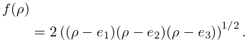
… ►The Weierstrass function $\mathrm{\wp }$ plays a similar role for cubic potentials in canonical form $g_3+g_{2}x-4x^3$. … ►Airault et al. (1977) applies the function $\mathrm{\wp }$ to an integrable classical many-body problem, and relates the solutions to nonlinear partial differential equations. … ►where $x,y,z$ are the corresponding Cartesian coordinates and $e_1$, $e_2$, $e_3$ are constants. … ►

23.21.3 $$f(\rho )=2{\left((\rho -e_1)(\rho -e_2)(\rho -e_3)\right)}^{1/2}.$$

ⓘ

Symbols:

$e_j$: Weierstrass lattice roots, $𝕃$: lattice, $\rho$: roots and $f(\rho )$: function

Permalink:

http://dlmf.nist.gov/23.21.E3

Encodings:

pMML, png, TeX

See also:

Annotations for §23.21(iii), §23.21 and Ch.23

►Another form is obtained by identifying $e_1$, $e_2$, $e_3$ as lattice roots (§23.3(i)), and setting …

15: 23.4 Graphics

… ►

§23.4(i) Real Variables

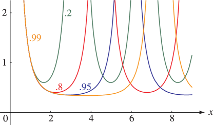
►Line graphs of the Weierstrass functions $\mathrm{\wp }\left(x\right)$, $\zeta \left(x\right)$, and $\sigma \left(x\right)$, illustrating the lemniscatic and equianharmonic cases. … ►

►►

Figure 23.4.7: $\mathrm{\wp }\left(x\right)$ with ${\omega }_1=K\left(k\right)$, ${\omega }_3=\mathrm{i}{K}^{\prime }\left(k\right)$ for $0\le x\le 9$, $k^2$ = 0. … Magnify

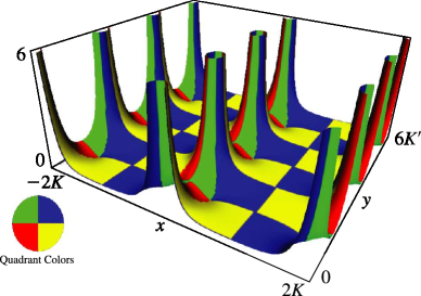
… ►Surfaces for the Weierstrass functions $\mathrm{\wp }\left(z\right)$, $\zeta \left(z\right)$, and $\sigma \left(z\right)$. … ►

►

►

Figure 23.4.8: $\mathrm{\wp }\left(x+\mathrm{i}y\right)$ with ${\omega }_1=K\left(k\right)$, ${\omega }_3=\mathrm{i}{K}^{\prime }\left(k\right)$ for $-2K\left(k\right)\le x\le 2K\left(k\right)$, $0\le y\le 6K^{\prime }\left(k\right)$, $k^2=0.9$. (The scaling makes the lattice appear to be square.) Magnify 3D Help

…

16: 26.5 Lattice Paths: Catalan Numbers

§26.5 Lattice Paths: Catalan Numbers

►

§26.5(i) Definitions

… ►It counts the number of lattice paths from $(0,0)$ to $(n,n)$ that stay on or above the line $y=x$. … ►

Table 26.5.1: Catalan numbers.

► ►►►

$n$	$C\left(n\right)$	$n$	$C\left(n\right)$	$n$	$C\left(n\right)$
…
6	132	13	7 42900	20	65641 20420

►

…

17: 23.5 Special Lattices

§23.5 Special Lattices

… ►

§23.5(ii) Rectangular Lattice

… ►

§23.5(iii) Lemniscatic Lattice

… ►

§23.5(iv) Rhombic Lattice

… ►

§23.5(v) Equianharmonic Lattice

…

18: 23.23 Tables

… ►2 in Abramowitz and Stegun (1964) gives values of $\mathrm{\wp }\left(z\right)$, ${\mathrm{\wp }}^{\prime }\left(z\right)$, and $\zeta \left(z\right)$ to 7 or 8D in the rectangular and rhombic cases, normalized so that ${\omega }_1=1$ and ${\omega }_3=\mathrm{i}a$ (rectangular case), or ${\omega }_1=1$ and ${\omega }_3=\frac{1}{2}+\mathrm{i}a$ (rhombic case), for $a$ = 1. …05, and in the case of $\mathrm{\wp }\left(z\right)$ the user may deduce values for complex $z$ by application of the addition theorem (23.10.1). ►Abramowitz and Stegun (1964) also includes other tables to assist the computation of the Weierstrass functions, for example, the generators as functions of the lattice invariants $g_2$ and $g_3$. …

19: 29.2 Differential Equations

… ►This equation has regular singularities at the points $2pK+(2q+1)\mathrm{i}{K}^{\prime }$, where $p,q\in \mathbb{Z}$, and $K$, $K^{\prime }$ are the complete elliptic integrals of the first kind with moduli $k$, $k^{\prime }(={(1-k^2)}^{1/2})$, respectively; see §19.2(ii). In general, at each singularity each solution of (29.2.1) has a branch point (§2.7(i)). … ►

29.2.9 $$\frac{d^{2}w}{{d\eta }^2}+(g-\nu (\nu +1)\mathrm{\wp }\left(\eta \right))w=0,$$

ⓘ

Symbols:

$\mathrm{\wp }\left(z\right)$ (= $\mathrm{\wp }\left(z|𝕃\right)$ = $\mathrm{\wp }(z;g_2,g_3)$): Weierstrass $\mathrm{\wp }$-function, $\frac{df}{dx}$: derivative of $f$ with respect to $x$ , $\nu$: real parameter, $g$ and $\eta$

Permalink:

http://dlmf.nist.gov/29.2.E9

Encodings:

pMML, png, TeX

See also:

Annotations for §29.2(ii), §29.2 and Ch.29

… ►

29.2.11 $$\zeta =\mathrm{\wp }(\eta ;g_2,g_3)=\mathrm{\wp }\left(\eta \right),$$

ⓘ

Defines:

$\zeta$ (locally)

Symbols:

$\mathrm{\wp }(z;g_2,g_3)$: Weierstrass $\mathrm{\wp }$-function, $\mathrm{\wp }\left(z\right)$ (= $\mathrm{\wp }\left(z|𝕃\right)$ = $\mathrm{\wp }(z;g_2,g_3)$): Weierstrass $\mathrm{\wp }$-function, $\eta$ , $g_2$ and $g_3$

Permalink:

http://dlmf.nist.gov/29.2.E11

Encodings:

pMML, png, TeX

See also:

Annotations for §29.2(ii), §29.2 and Ch.29

…

20: 20.7 Identities

… ►

20.7.15 $$A\equiv A(\tau )=1/{\theta }_4\left(0\right|2\tau ),$$

ⓘ

Defines:

$A$ (locally)

Symbols:

${\theta }_j\left(z\right|\tau )$: theta function, $\equiv$: equals by definition and $\tau$: lattice parameter

Permalink:

http://dlmf.nist.gov/20.7.E15

Encodings:

pMML, png, TeX

See also:

Annotations for §20.7(vi), §20.7 and Ch.20

… ►See Lawden (1989, pp. 19–20). … ►

§20.7(viii) Transformations of Lattice Parameter

… ►

20.7.28 $${\theta }_3\left(z\right|\tau +1)={\theta }_4\left(z\right|\tau ),$$

ⓘ

Symbols:

${\theta }_j\left(z\right|\tau )$: theta function, $z$: complex and $\tau$: lattice parameter

Permalink:

http://dlmf.nist.gov/20.7.E28

Encodings:

pMML, png, TeX

See also:

Annotations for §20.7(viii), §20.7 and Ch.20

►

20.7.29 $${\theta }_4\left(z\right|\tau +1)={\theta }_3\left(z\right|\tau ).$$

ⓘ

Symbols:

${\theta }_j\left(z\right|\tau )$: theta function, $z$: complex and $\tau$: lattice parameter

Permalink:

http://dlmf.nist.gov/20.7.E29

Encodings:

pMML, png, TeX

See also:

Annotations for §20.7(viii), §20.7 and Ch.20

…