invariants
(0.000 seconds)
21—30 of 38 matching pages
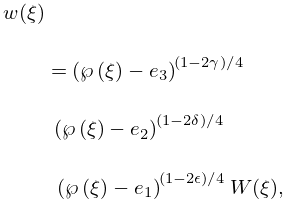
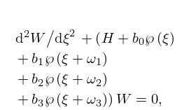
21: 29.2 Differential Equations
22: 23.22 Methods of Computation
…
►The modular functions , , and are also obtainable in a similar manner from their definitions in §23.15(ii).
…
►The corresponding values of , , are calculated from (23.6.2)–(23.6.4), then and are obtained from (23.3.6) and (23.3.7).
►
Starting from Invariants
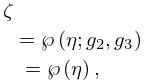
►Suppose that the invariants , , are given, for example in the differential equation (23.3.10) or via coefficients of an elliptic curve (§23.20(ii)). … ►Assume and . …23: 23.20 Mathematical Applications
…
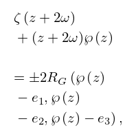
►Points on the curve can be parametrized by , , where and : in this case we write .
…
24: 31.2 Differential Equations
25: 19.25 Relations to Other Functions
…
►then the five nontrivial permutations of that leave
invariant change () into , , , , , and () into , , , , .
…
►
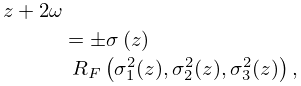
19.25.36
…
►
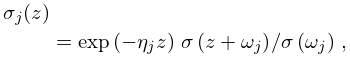
19.25.37
…
►
19.25.40
…
►
19.25.41
…
26: Bibliography V
…
►
On the coefficients of the modular invariant
.
Nederl. Akad. Wetensch. Proc. Ser. A. 56 = Indagationes
Math. 15 56, pp. 389–400.
…
27: Bibliography P
…
►
Unbiasedness of invariant tests for MANOVA and other multivariate problems.
Ann. Statist. 8 (6), pp. 1326–1341.
…
28: 28.5 Second Solutions ,
…
►(Other normalizations for and can be found in the literature, but most formulas—including connection formulas—are unaffected since and are invariant.)
…
29: Bibliography
…
►
Conformal Invariants, Inequalities, and Quasiconformal Maps.
John Wiley & Sons Inc., New York.
…
