integral%20equation%20for%20Lam%C3%A9%20functions

SearchAdvancedHelp

(0.008 seconds)

11—20 of 989 matching pages

11: 15.10 Hypergeometric Differential Equation

… ►

15.10.1 $$z(1-z)\frac{d^{2}w}{{dz}^2}+\left(c-(a+b+1)z\right)\frac{dw}{dz}-abw=0.$$

ⓘ

Symbols:

$\frac{df}{dx}$: derivative of $f$ with respect to $x$ , $z$: complex variable, $a$: real or complex parameter, $b$: real or complex parameter and $c$: real or complex parameter

Referenced by:

§15.11(i), §15.11(i), §15.17(ii), §15.19(ii), §15.2(ii), §15.5(ii), §16.13, §17.6(iv), §19.18(ii), §19.4(ii)

Permalink:

http://dlmf.nist.gov/15.10.E1

Encodings:

pMML, png, TeX

See also:

Annotations for §15.10(i), §15.10 and Ch.15

… ►

Singularity $z=0$

… ►

Singularity $z=1$

… ►

Singularity $z=\mathrm{\infty }$

… ►The $\left(\genfrac{}{}{0.0pt}{}{6}{3}\right)=20$ connection formulas for the principal branches of Kummer’s solutions are: …

12: 30.2 Differential Equations

§30.2 Differential Equations

►

§30.2(i) Spheroidal Differential Equation

… ► … ►The Liouville normal form of equation (30.2.1) is … ►If $\gamma =0$, Equation (30.2.4) is satisfied by spherical Bessel functions; see (10.47.1).

13: 36.2 Catastrophes and Canonical Integrals

§36.2 Catastrophes and Canonical Integrals

… ►

Canonical Integrals

… ► ${\mathrm{\Psi }}_1$ is related to the Airy function (§9.2): … … ►

§36.2(iii) Symmetries

…

14: 28.2 Definitions and Basic Properties

… ►

28.2.1 $$w^{\prime \prime }+(a-2q\cos \left(2z\right))w=0.$$

ⓘ

Symbols:

$\cos z$: cosine function, $q=h^2$: parameter, $z$: complex variable, $a$: parameter and $w(z)$: Mathieu’s equation solution

A&S Ref:

20.3.1 20.1.1 (in slightly different form)

Referenced by:

§1.18(vii), Figure 28.17.1, Figure 28.17.1, §28.17, §28.17, §28.2(ii), §28.2(ii), §28.2(iii), §28.2(iv), §28.20(i), §28.29(i), §28.32(i), §28.32(i), 1st item, 2nd item, §28.33(iii), item (a), item (c), item (c), §28.5(i), §28.8(iv), §28.8(iv), §28.8(iv), §30.2(iii)

Permalink:

http://dlmf.nist.gov/28.2.E1

Encodings:

pMML, png, TeX

See also:

Annotations for §28.2(i), §28.2 and Ch.28

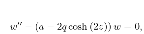
… ►This is the characteristic equation of Mathieu’s equation (28.2.1). … ►

§28.2(iv) Floquet Solutions

… ►

§28.2(vi) Eigenfunctions

… ►For simple roots $q$ of the corresponding equations (28.2.21) and (28.2.22), the functions are made unique by the normalizations …

15: 32.2 Differential Equations

§32.2 Differential Equations

… ►The six Painlevé equations ${\text{P}}_{\text{I}}$–${\text{P}}_{\text{VI}}$ are as follows: … ►The fifty equations can be reduced to linear equations, solved in terms of elliptic functions (Chapters 22 and 23), or reduced to one of ${\text{P}}_{\text{I}}$–${\text{P}}_{\text{VI}}$. … ►

§32.2(ii) Renormalizations

… ► …

16: 28.20 Definitions and Basic Properties

… ►

§28.20(i) Modified Mathieu’s Equation

►When $z$ is replaced by $\pm \mathrm{i}z$, (28.2.1) becomes the modified Mathieu’s equation: ►

28.20.1 $$w^{\prime \prime }-\left(a-2q\cosh \left(2z\right)\right)w=0,$$

ⓘ

Symbols:

$\cosh z$: hyperbolic cosine function, $q=h^2$: parameter, $z$: complex variable, $a$: parameter and $w(z)$: Mathieu’s equation solution

A&S Ref:

20.1.2 (in slightly different form) 20.8.6

Referenced by:

§28.20(iii), §28.32(i), 1st item, 2nd item, item (b), §28.8(iv), §28.8(iv)

Permalink:

http://dlmf.nist.gov/28.20.E1

Encodings:

pMML, png, TeX

See also:

Annotations for §28.20(i), §28.20 and Ch.28

… ►Then from §2.7(ii) it is seen that equation (28.20.2) has independent and unique solutions that are asymptotic to ${\zeta }^{1/2}{\mathrm{e}}^{\pm 2\mathrm{i}h\zeta }$ as $\zeta \to \mathrm{\infty }$ in the respective sectors $|\mathrm{ph}\left(\mp \mathrm{i}\zeta \right)|\le \frac{3}{2}\pi -\delta$, $\delta$ being an arbitrary small positive constant. … ►

§28.20(iv) Radial Mathieu Functions ${\mathrm{Mc}}_n^{(j)}$, ${\mathrm{Ms}}_n^{(j)}$

…

17: 8.26 Tables

… ►

Khamis (1965) tabulates $P(a,x)$ for $a=0.05(.05)10(.1)20(.25)70$, $0.0001\le x\le 250$ to 10D.

… ►

§8.26(iv) Generalized Exponential Integral

►

Abramowitz and Stegun (1964, pp. 245–248) tabulates $E_n\left(x\right)$ for $n=2,3,4,10,20$, $x=0(.01)2$ to 7D; also $(x+n){\mathrm{e}}^x{E}_n\left(x\right)$ for $n=2,3,4,10,20$, $x^{-1}=0(.01)0.1(.05)0.5$ to 6S.

… ►

Pagurova (1961) tabulates $E_n\left(x\right)$ for $n=0(1)20$, $x=0(.01)2(.1)10$ to 4-9S; ${\mathrm{e}}^x{E}_n\left(x\right)$ for $n=2(1)10$, $x=10(.1)20$ to 7D; ${\mathrm{e}}^x{E}_p\left(x\right)$ for $p=0(.1)1$, $x=0.01(.01)7(.05)12(.1)20$ to 7S or 7D.

… ►

Zhang and Jin (1996, Table 19.1) tabulates $E_n\left(x\right)$ for $n=1,2,3,5,10,15,20$, $x=0(.1)1,1.5,2,3,5,10,20,30,50,100$ to 7D or 8S.

18: 36 Integrals with Coalescing Saddles

Chapter 36 Integrals with Coalescing Saddles

…

19: 20 Theta Functions

Chapter 20 Theta Functions

…

20: 6.19 Tables

… ►

§6.19(ii) Real Variables

►

Abramowitz and Stegun (1964, Chapter 5) includes $x^{-1}\mathrm{Si}\left(x\right)$, $-x^{-2}\mathrm{Cin}\left(x\right)$, $x^{-1}\mathrm{Ein}\left(x\right)$, $-x^{-1}\mathrm{Ein}\left(-x\right)$, $x=0(.01)0.5$; $\mathrm{Si}\left(x\right)$, $\mathrm{Ci}\left(x\right)$, $\mathrm{Ei}\left(x\right)$, $E_1\left(x\right)$, $x=0.5(.01)2$; $\mathrm{Si}\left(x\right)$, $\mathrm{Ci}\left(x\right)$, $x{\mathrm{e}}^{-x}\mathrm{Ei}\left(x\right)$, $x{\mathrm{e}}^x{E}_1\left(x\right)$, $x=2(.1)10$; $x\mathrm{f}\left(x\right)$, $x^2\mathrm{g}\left(x\right)$, $x{\mathrm{e}}^{-x}\mathrm{Ei}\left(x\right)$, $x{\mathrm{e}}^x{E}_1\left(x\right)$, $x^{-1}=0(.005)0.1$; $\mathrm{Si}\left(\pi x\right)$, $\mathrm{Cin}\left(\pi x\right)$, $x=0(.1)10$. Accuracy varies but is within the range 8S–11S.

►

Zhang and Jin (1996, pp. 652, 689) includes $\mathrm{Si}\left(x\right)$, $\mathrm{Ci}\left(x\right)$, $x=0(.5)20(2)30$, 8D; $\mathrm{Ei}\left(x\right)$, $E_1\left(x\right)$, $x=[0,100]$, 8S.

… ►

Abramowitz and Stegun (1964, Chapter 5) includes the real and imaginary parts of $z{\mathrm{e}}^z{E}_1\left(z\right)$, $x=-19(1)20$, $y=0(1)20$, 6D; ${\mathrm{e}}^z{E}_1\left(z\right)$, $x=-4(.5)-2$, $y=0(.2)1$, 6D; $E_1\left(z\right)+\ln z$, $x=-2(.5)2.5$, $y=0(.2)1$, 6D.

►

Zhang and Jin (1996, pp. 690–692) includes the real and imaginary parts of $E_1\left(z\right)$, $\pm x=0.5,1,3,5,10,15,20,50,100$, $y=0(.5)1(1)5(5)30,50,100$, 8S.